. 2010 Sep 10:4:23.
doi: 10.3389/fncom.2010.00023. eCollection 2010.

STDP in Recurrent Neuronal Networks

Affiliations

STDP in Recurrent Neuronal Networks

Matthieu Gilson et al. Front Comput Neurosci. .

Abstract

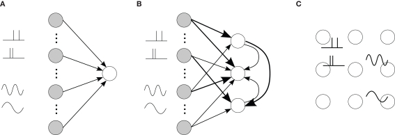
Recent results about spike-timing-dependent plasticity (STDP) in recurrently connected neurons are reviewed, with a focus on the relationship between the weight dynamics and the emergence of network structure. In particular, the evolution of synaptic weights in the two cases of incoming connections for a single neuron and recurrent connections are compared and contrasted. A theoretical framework is used that is based upon Poisson neurons with a temporally inhomogeneous firing rate and the asymptotic distribution of weights generated by the learning dynamics. Different network configurations examined in recent studies are discussed and an overview of the current understanding of STDP in recurrently connected neuronal networks is presented.

Keywords: STDP; network structure; recurrent neuronal network; self-organization / unsupervised learning; spike-time correlations.


Figures

Figure 1
Figure 1
(A) Schematic representation of a synapse from the source neuron j to the target neuron i. The synaptic weight is Jij and axonal delay dijax; dijden accounts for the conduction of the postsynaptic response along the dendritic tree toward the soma while the dijb accounts for the back-propagation of action potential to the synapse. Here dijden and dijb are distinguished, but they can be considered to be equal if the conduction along the dendrite in both directions is passive. (B) Examples of STDP learning window function; the vertical scale (dimensionless) indicates the change of synaptic strength arising from the occurrence of a pair of pre- and postsynaptic spikes with time difference u. The darker curves correspond to stronger values for the current weight, indicating the effect of weight dependence.
Figure 2
Figure 2
(A) Single neuron. Spike-timing-dependent plasticity (STDP) refers to the development of synaptic weights Jij (small filled circles, 1 ≤ j ≤ N) of a single neuron (large circle) in dependence upon the arrival times of presynaptic spikes (input) and firing times of the postsynaptic neuron (output). Here the neuron receives input spike trains denoted by Sj and produces output spikes denoted by Si. The collective interaction of all the input spikes determines the firing times of the postsynaptic neuron they are all sitting on and in this way the input spike times at different synapses influence the latter's waxing and waning. (B) Recurrently connected network. Schematic representation of two neurons i and j stimulated by one external input k with spike train S^k. Input and recurrent weights are denoted by K and J, respectively.
Figure 3
Figure 3
Evolution of synaptic weights. In each plot individual weights are represented (gray traces) as well as their overall mean Jav (thick solid black line) and the two means over each input pool (thick dashed and dashed-dotted black lines). In the simulations, one pool had spike-time correlation while the other had none while win = win = 0. (A) Case of non-realizable (but stable) fixed point Jav*<0. (B) Stability of the mean incoming weight (0=Jmin<Jav*<Jmax=0.06) and competition between individual weights when using almost-additive STDP. (C) Similar plot to (B) with medium weight dependence, which implies weaker competition.
Figure 4
Figure 4
Spike-time correlograms between (A) two inputs, (B) an input and a neuron, and (C) two neurons. These three plots correspond to Eq. 6 for randomly chosen pairs of inputs/neurons in a network of 100 neurons excited by 100 inputs (30% probability of connection; no learning was applied) and simulated over 1000 s with the sum of delays dijax+dijden=4 ms; the time bin is 2 ms. (D) Learning window function W(Jav*,u) with no delay (solid line, Δdij = 0 ms), purely dendritic delay dijb=4 ms (dashed line, Δdij = −4 ms) and purely axonal delay dijax=4 ms (dashed-dotted line, Δdij = 4 ms). (E,F) Theoretical curves of ψ and ζ corresponding to approximation at the first order of the correlograms in (B,C), respectively, with short (4 ms, solid lines) and large (10 ms, dashed lines) values for dijax+dijden; cf. Eq. 8. The two curves (for 4 and 10 ms) are superimposed for ζ and the thin lines represent the corresponding predictions when incorporating a further order in the recurrent connectivity. The agreement with the spreading and amplitude of the curves in (B,C), which correspond to 4 ms, is only qualitative
Figure 5
Figure 5
Four illustrative plots of the STDP learning window W (gray solid line) and its convolutions in Eq. 9: W*ψ for input connections (dashed line) and W*ζ for recurrent connections (dashed-dotted line). The theoretical spike-time correlograms ψ and ζ in Eq. 8 can be found in Figures 4E,F, respectively. The sign of the function resulting from the convolution for the argument Δdij predicts the weight evolution. The curves correspond to delays such that dijax+dijden=4 ms and the effect of Δdij can be read on the horizontal axis (technically, it should be read −4 ≤ Δdij ≤ 4). Comparison between an STDP learning window W(Jav*,u) that induces (A) more potentiation than depression for small values of u and (B) the converse situation. We note that the integral is negative in both cases, which means more overall depression (for uncorrelated inputs), which is required for stability. (C,D) Similar plots to (A,B) with a discontinuous curve W in u = 0.
Figure 6
Figure 6
Self-organization scheme in a network (top circles) stimulated by two correlated pools of external inputs (bottom circles). The diagrams represent the connectivity before and after learning (indicated by the block arrows, ⇒ and ⇐). For initial configurations, thin arrows represent fixed connections while thick arrows denote plastic connections. After learning, very thick (resp. dashed) arrows indicate potentiated (depressed) weights. In case (C) two different network topologies that can emerge are represented, depending on the particular learning and neuronal parameters. A mathematical analysis of the weight dynamics for configurations in (A), (B), (C,D), and (E) can be found in Gilson et al. (2009a), Gilson et al. (2009b), Gilson et al. (2009d), and Gilson et al. (2010), respectively.
Figure 7
Figure 7
Spike-time cross-correlograms Cij(·,u) for 2 out of 100 recurrently connected neurons with 30% probability that receive (A) oscillatory stimulation at 100 Hz and (B) pacemaker-like activity (regular pulse train at 25 Hz). Both input and recurrent delays were chosen equal to 4 ± 1 ms (uniformly distributed in the interval [3,5] ms).
Figure 8
Figure 8
Typical connectivity matrices for recurrent connections (A) before and (B) after a learning epoch during which the weight specialization due to STDP corresponds to Figure 6C(⇒). Darker pixels indicate stronger weights. (C) Resulting spike-time correlograms for two neurons within the same emerged group in the recurrently connected network that only receives spontaneous (homogeneous) excitation before (dashed curve) and after (solid curve) the above mentioned weight specialization. These neurons do not have direct synaptic connections between each other. (D) Similar to (C) with external stimulation from two delta-correlated pools similar to Figure 6C. (E) Connectivity matrix corresponding to three groups forming a feed-forward loop. (F) Spike-time correlogram (averaged over several neurons) between two successively connected groups when the first group receives correlated external stimulation.
Figure 9
Figure 9
(A) Single neuron (open circle) excited by external input neurons (filled circles) that correspond to specific spike-time correlation structure, such as oscillatory activity and spike patterns. The four thumbnail sketches on the LHS of the plot represent two different types of input correlation structure: inputs containing a repeated spike patterns (top two thumbnails) and inputs with an oscillating firing rate (bottom two thumbnails). (B) Strengthening of some input and recurrent connections (thick arrows) for several such neurons. (C) Resulting specialization of some areas (neighbor neurons) in the network to some of the presented stimuli (thumbnails), which implies differentiated topological spiking activity depending on the presented stimulus. External inputs are not represented in (C).

Similar articles

Cited by

References

    1. Amit D. J., Brunel N. (1997). Dynamics of a recurrent network of spiking neurons before and following learning. Netw. Comput. Neural Syst. 8, 373–40410.1088/0954-898X/8/4/003 - DOI
    1. Appleby P. A., Elliott T. (2006). Stable competitive dynamics emerge from multispike interactions in a stochastic model of spike-timing-dependent plasticity. Neural Comput. 18, 2414–246410.1162/neco.2006.18.10.2414 - DOI - PubMed
    1. Appleby P. A., Elliott T. (2007). Multispike interactions in a stochastic model of spike-timing-dependent plasticity. Neural Comput. 19, 1362–139910.1162/neco.2007.19.5.1362 - DOI - PubMed
    1. Bartsch A. P., van Hemmen J. L. (2001). Combined Hebbian development of geniculocortical and lateral connectivity in a model of primary visual cortex. Biol. Cybern. 84, 41–5510.1007/s004220170003 - DOI - PubMed
    1. Bi G. Q., Poo M. M. (1998). Synaptic modifications in cultured hippocampal neurons: dependence on spike timing, synaptic strength, and postsynaptic cell type. J. Neurosci. 18, 10464–10472 - PMC - PubMed

LinkOut - more resources