Coupled noisy spiking neurons as velocity-controlled oscillators in a model of grid cell spatial firing

Abstract

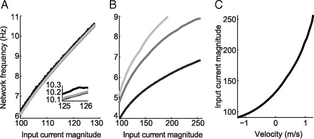
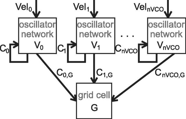
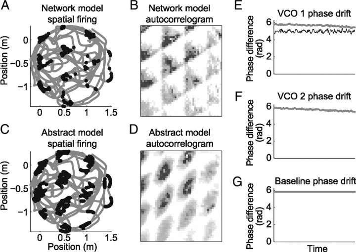
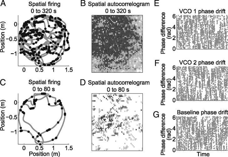
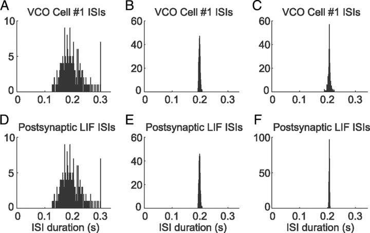
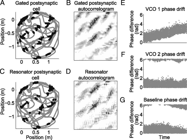
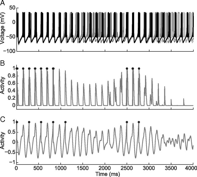
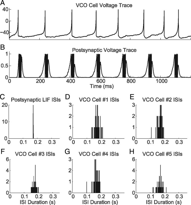
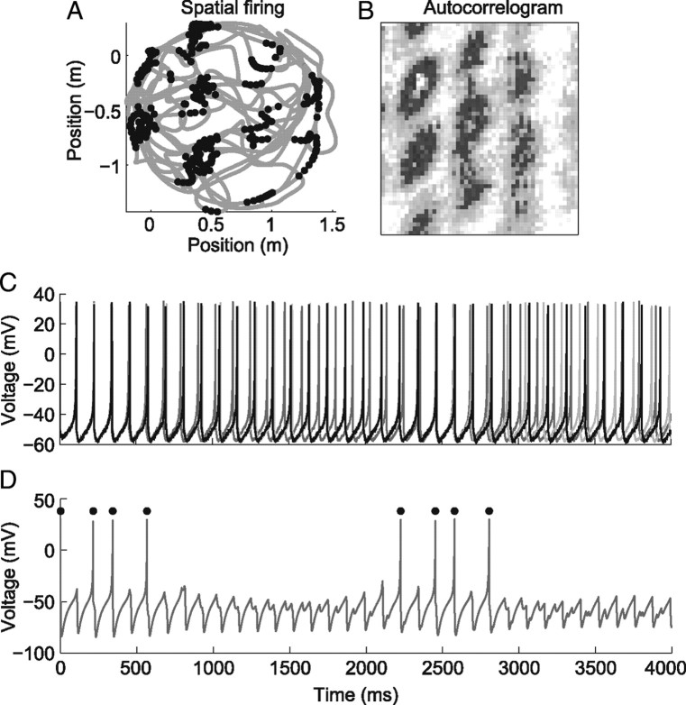
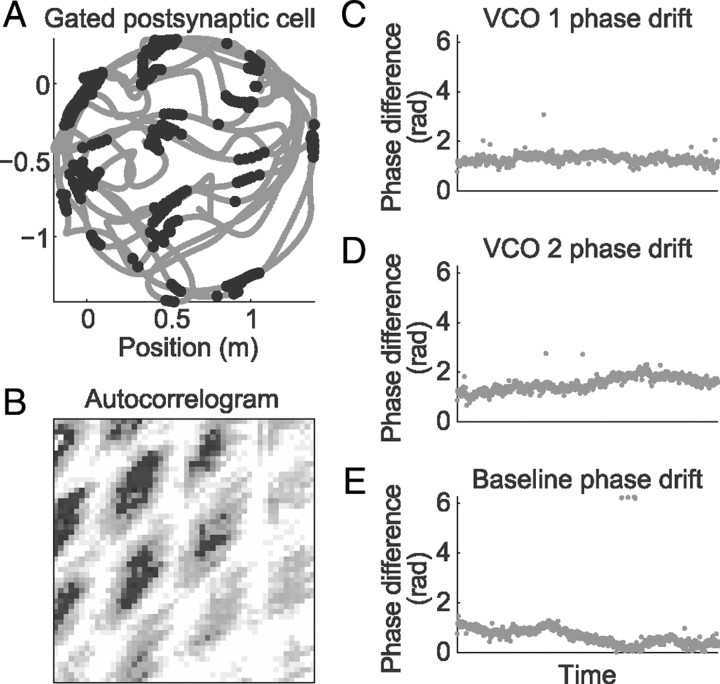
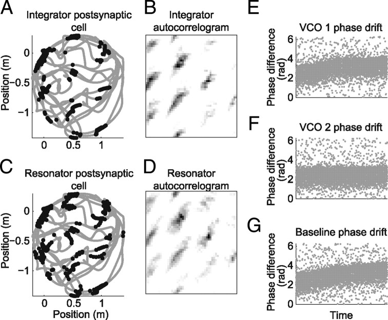
One of the two primary classes of models of grid cell spatial firing uses interference between oscillators at dynamically modulated frequencies. Generally, these models are presented in terms of idealized oscillators (modeled as sinusoids), which differ from biological oscillators in multiple important ways. Here we show that two more realistic, noisy neural models (Izhikevich's simple model and a biophysical model of an entorhinal cortex stellate cell) can be successfully used as oscillators in a model of this type. When additive noise is included in the models such that uncoupled or sparsely coupled cells show realistic interspike interval variance, both synaptic and gap-junction coupling can synchronize networks of cells to produce comparatively less variable network-level oscillations. We show that the frequency of these oscillatory networks can be controlled sufficiently well to produce stable grid cell spatial firing on the order of at least 2-5 min, despite the high noise level. Our results suggest that the basic principles of oscillatory interference models work with more realistic models of noisy neurons. Nevertheless, a number of simplifications were still made and future work should examine increasingly realistic models.

Figure 1.

Firing frequency versus input current for individual and networks of simple model cells. A, The firing frequency of an individual cell without noise (light gray) is very similar to the response of an individual noisy cell (black), but even more similar to a network of 250 noisy, gap-junction-coupled neurons (dark gray). For clarity, an inset with an expanded y-axis is shown. B, A network of 250 noisy, synaptically coupled neurons fires at much lower frequencies than any of the cells in A for the same input magnitude. The entire F(I) curve also moves downward as the synaptic coupling strength g is increased (g = 192, light gray; g = 256, dark gray; g = 384, black) (compare with supplemental Fig. S4A, available at www.jneurosci.org as supplemental material). C, Since the firing rate, f, is directly related to velocity, v, v = (f − ω_b)/β, the inverse of the F(I) curve (shown for the synaptically coupled network) describes the input an oscillator network requires to encode different velocities along its preferred direction. General parameters: 15 s simulations and see Table 1. Single unit: n = 1, w = 1.2, σ = 0, or σ = 100. Gap-junction coupling: n = 250, w = 0.0048, σ = 100. Synaptic coupling: n = 250, w = 0.0048, σ = 100, ω_b = 6.4405 Hz.

Figure 2.

Architecture of the model. The input to the model is a set of n_VCO + 1 velocity signals, Vel_i. These signals go to respective networks V_i that are all-to-all internally coupled over connections C_i, which may be either synapses or gap junctions. The grid cell G receives input over synapses C_i,G from all cells in all V_i.

Figure 3.

Two-dimensional grid cell with oscillators comprising single, noise-free simple model neurons. A, The network receives velocity input corresponding to a smooth two-dimensional trajectory (gray) and a leaky integrator postsynaptic cell generates spikes (black) as output. B, The autocorrelogram of the spatial firing in A shows the clear hexagonal pattern characteristic of grid cells. C, D, A simulation of the abstract model produces essentially identical results to A and B apart from spatial displacement and difference in field size. E, F, Phase differences between simple model and abstract model of the two active velocity-controlled oscillators show a linear drift over time, and the fluctuations correspond to the velocities along the preferred directions of the respective VCOs. E, Black line, For comparison, the horizontal component of velocity that is encoded by VCO 1. G, The baseline oscillators accumulate no phase error in this noiseless simulation. Parameters: 320 s simulation, n_VCO = 2 (active VCO preferred directions of 0 and 2π/3 radians), n = 1, τ = 40 ms, w₀ = 0.8, w₁ = 0.14, ω_b = 7.8989 Hz; Table 1.

Figure 4.

Noisy simple model neurons, when uncoupled, are unfit as oscillators. A, C, The network receives velocity input corresponding to a smooth two-dimensional trajectory (gray), and the locations where the simulated grid cell spikes over the entire 320 s (A) and first 80 s (C) are indicated with black dots. B, D, The autocorrelogram of the spatial firing shows no clear regularity, even early in the simulation. E–G, Phase differences between corresponding oscillators show that realistically noisy neurons lose their correct phases very quickly compared with behavioral timescales. Parameters: 320 s simulation, n_VCO = 2 [active VCO preferred directions of 0 and 2π/3 radians], n = 1, σ = 100, τ = 40 ms, w₀ = 0.8, w₁ = 0.14, ω_b = 7.8989 Hz; Table 1.

Figure 5.

ISI histograms for cells in three conditions. A, ISIs of an uncoupled, noisy simple model neuron are much more variable than when multiple cells are coupled (as in B and C). B, ISIs of one noisy neuron from a network of 250 gap-junction-coupled neurons. C, ISIs of one noisy neuron from a network of 250 synaptically coupled neurons. D, ISIs of a LIF cell driven by the cell in A. The histograms are identical, showing that the postsynaptic cell directly inherits the variability of the cell driving it. E, ISIs of an LIF cell receiving input from all 250 gap-junction-coupled neurons. The variability of individual gap-junction-coupled neurons is very similar to the variability of the postsynaptic cell. F, ISIs of an LIF cell receiving input from all 250 synaptically coupled neurons. The individual cells (C) are noticeably more variable than the postsynaptic cell (and see Fig. 8 for a more extreme case). Parameters: 60 s simulations, n = 1 (w = 1.2) or n = 250 (w = 0.0048), σ = 100; Table 1.

Figure 6.

Two-dimensional grid cell with network oscillators made of noisy, synaptically coupled simple model neurons. A, The network receives velocity input corresponding to a smooth two-dimensional trajectory (gray) and a gated, leaky integrator postsynaptic cell generates spikes (black). B, The autocorrelogram of the spatial firing in A shows hexagonal periodicity. Parameters: t_gate = 0.001 s, τ = 5 ms, w = 0.0016. C, D, The spatial firing and spatial autocorrelogram of the same network but with a resonant postsynaptic cell. Parameters: c_res = −0.01, ω_res = ω_b, w₀ = 0.0024, w₁ = w₂ = 0.002. E–G, Phase differences between network and abstract models of the two active velocity-controlled oscillators. The average of the phase differences remains relatively constant, although individual cells are firing over a much wider range of phases compared with when the cells are instead gap-junction-coupled. General parameters: 280 s simulation. n_VCO = 2 [active VCO preferred directions of 0 and 2π/3 radians], n = 250, σ = 100, ω_b = 7.2543 Hz; Table 1.

Figure 7.

Combining the activity of multiple synaptically coupled oscillators. A, Voltage traces of single neurons from V₀ (black), V₁ (light gray), and V₂ (dark gray) in the first 4 s of the trajectory shown in Figure 6. B, The neurons in A project onto an integrate-and-fire neuron where cells in V₀ do not produce activity, but instead open a gate allowing cells in V₁ and V₂ to produce depolarization and sometimes spikes (black). Parameters: t_gate = 0.001 s, τ = 5 ms, w = 0.0016. C, The neurons in A project onto a resonate-and-fire neuron with resonant frequency equal to the baseline frequency. Parameters: c_res = −0.01, ω_res = ω_b, w₀ = 0.0024, w₁ = w₂ = 0.002. General parameters: n_VCO = 2 (active VCO preferred directions of 0 and 2π/3 radians), n = 250, σ = 100, ω_b = 7.2543 Hz; Table 1.

Figure 8.

A large network oscillator with a low connection probability can produce low-variance network oscillations while individual cells remain highly variable. A, Voltage trace over a short period of time of one of 5000 cells in a network where there is a 1% probability that any cell X connects to any other cell Y. The firing is irregular and the effects of noise are clear. B, Activity of postsynaptic integrate-and-fire cell receiving input from all 5000 oscillator cells including the one in A. The inputs to the postsynaptic cell are fairly spread out in time during each period so the cell fires in a burst. Comparing A to B, it can be seen that an individual cell will change its time of firing relative to the rest of the population on a cycle-by-cycle basis. C, A histogram of the ISIs of the postsynaptic cell from B shows that the period between bursts is highly consistent (period SD, 0.0008 s) despite the irregular inputs. This allows the oscillator to be used successfully in full spatial grid simulations (Fig. 11). D–H, ISI histograms for five cells in the network oscillators show the same mean ISI as the postsynaptic cell but much larger variability. The median period SD over all 5000 cells was 0.015 s, ∼20 times that of the postsynaptic cell in B and approximately half of the period SD of the uncoupled cells. Parameters: 10 s simulations, I = 95.8, n = 5000 cells, w = 0.0006, 1% connectivity; Table 1.

Figure 9.

Inhibitory noisy simple model neurons as oscillators. A, The network receives velocity input corresponding to a smooth two-dimensional trajectory (gray) and a spontaneously spiking simple model postsynaptic cell generates spikes (black). B, The autocorrelogram of the spatial firing in A demonstrates clear hexagonal periodicity. C, Voltage traces of single cells from gap-junction-coupled networks V₀ (light gray), V₁ (dark gray), and V₂ (black). D, The cells in each V_i project with inhibitory synapses onto a simple model cell firing at ω_b. When the V_i are out of phase, the cell is tonically inhibited, but when the V_i move into phase, there is enough time for the cell to fire between volleys of inhibition. Parameters: 320 s simulation, n_VCO = 2 (active VCO preferred directions of 0 and 2π/3 radians), n = 250, σ = 100, ω_b = 8.9735 Hz, w₀ = −3.2, w₁ = w₂ = −0.76; Table 1.

Figure 10.

Noisy biophysical neuron networks (synaptically coupled) produce usable velocity controlled oscillators. A, The grid cell is modeled as a gated, leaky integrate-and-fire cell and its spiking (black) is shown along a 2D trajectory (gray). B, The autocorrelogram of the spatial firing in A confirms the clear hexagonal periodicity. C–E, The phase differences for all oscillators remain fairly steady during the simulation, demonstrating that the biophysical model is capable of implementing the oscillatory interference mechanism. Parameters: 240 s simulation. n_VCO = 2 (active VCO preferred directions of 0 and 2π/3 radians), n = 250, g = 80, σ = 3.44, t_gate = 0.040 s, τ = 50 ms, w = 0.0024, ω_b = 8.9519 Hz; Table 1.

Figure 11.

Sparsely coupled simple model neuron networks as oscillators. A, The spatial trajectory (gray) provides the input to three oscillator networks of n = 5000 neurons with a 1% connectivity probability. Though the individual cells in the networks are highly variable (Fig. 8), the network-level variability is low so the integrate-and-fire postsynaptic cell spikes (black) in a stable grid pattern during the 240 s. Parameters: τ = 12 ms, w₀ = 0.00019, w₁ = w₂ = 0.00018. B, Spatial autocorrelogram of the spiking in A. C, The resonate-and-fire postsynaptic cell is also able to combine its inputs to produce a stable grid. Parameters: c_res = −0.01, w_res = ω_b, w = 0.001. D, Spatial autocorrelogram of the spiking in C. E–G, The highly variable individual oscillators spike over most phases, but the average phase of the network shows very little phase drift compared with the abstract model. Every 25th phase difference is plotted due to the large number of spikes. Parameters: 240 s simulation. n_VCO = 2 [active VCO preferred directions of 0 and 2π/3 radians], n = 5000, p = 0.01, g = 256, σ = 100, ω_b = 8.7942 Hz; Table 1.

References

1. Acker CD, Kopell N, White JA. Synchronization of strongly coupled excitatory neurons: relating network behavior to biophysics. J Comput Neurosci. 2003;15:71–90. - PubMed
1. Alonso A, Klink R. Differential electroresponsiveness of stellate and pyramidal-like cells of medial entorhinal cortex layer II. J Neurophysiol. 1993;70:128–143. - PubMed
1. Ang CW, Carlson GC, Coulter DA. Hippocampal CA1 circuitry dynamically gates direct cortical inputs preferentially at theta frequencies. J Neurosci. 2005;25:9567–9580. - PMC - PubMed
1. Barry C, Hayman R, Burgess N, Jeffery KJ. Experience-dependent rescaling of entorhinal grids. Nat Neurosci. 2007;10:682–684. - PubMed
1. Blair HT, Welday AC, Zhang K. Scale-invariant memory representations emerge from moiré interference between grid fields that produce theta oscillations: a computational model. J Neurosci. 2007;27:3211–3229. - PMC - PubMed
Publication types