Timing of cochlear responses inferred from frequency-threshold tuning curves of auditory-nerve fibers

Abstract

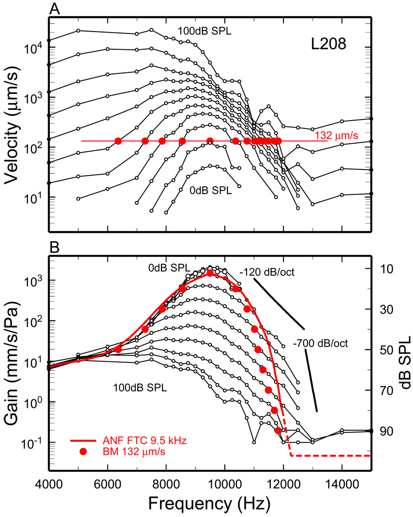
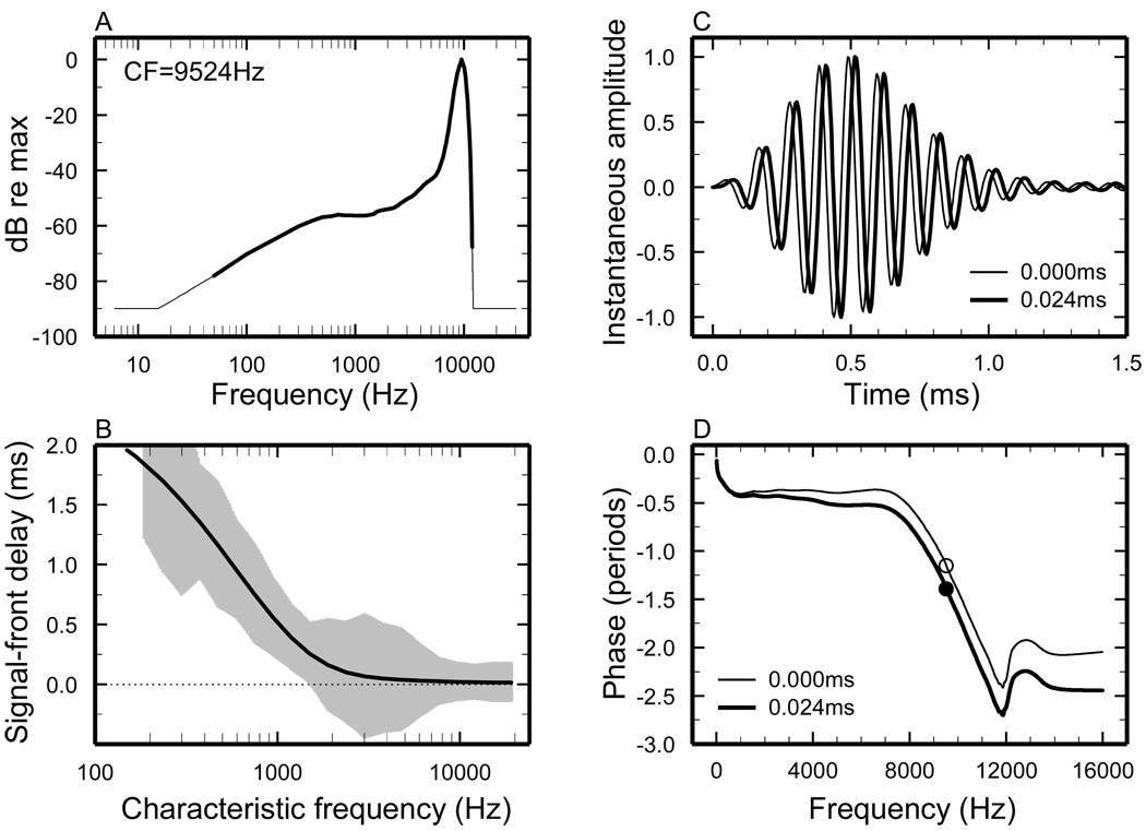
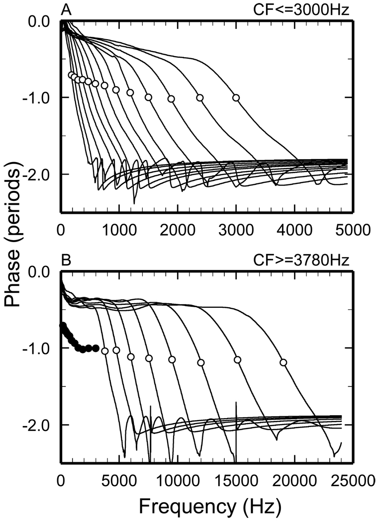
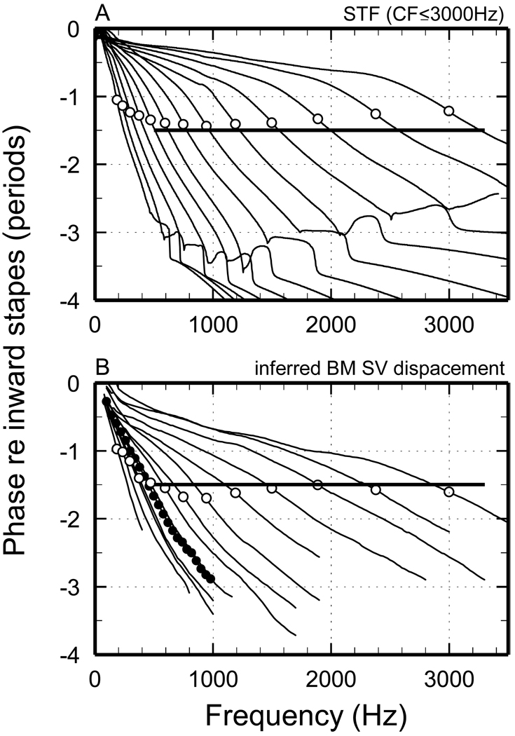
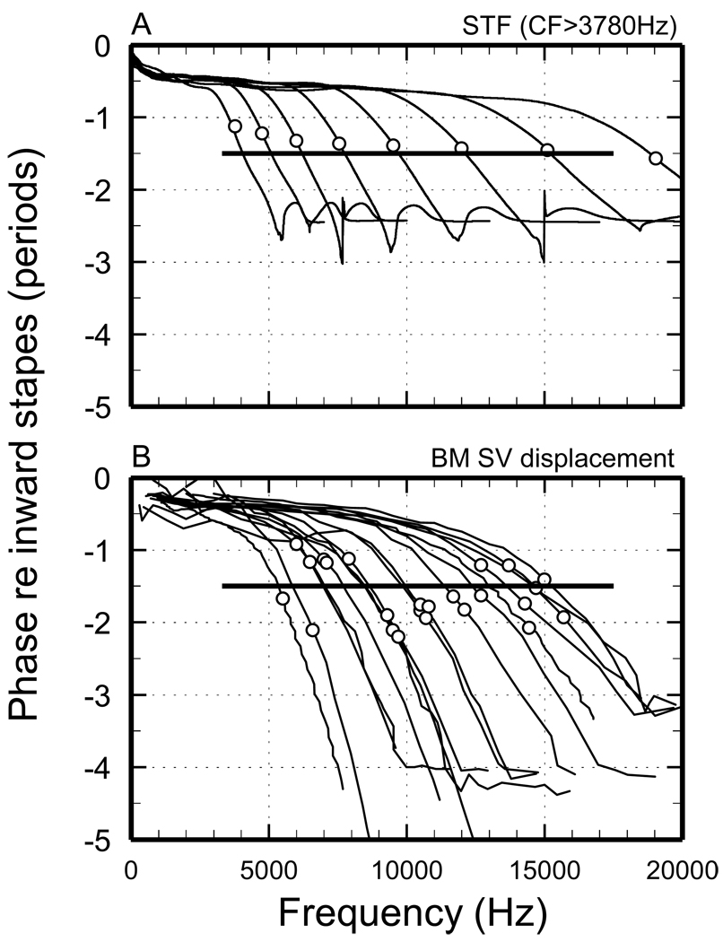
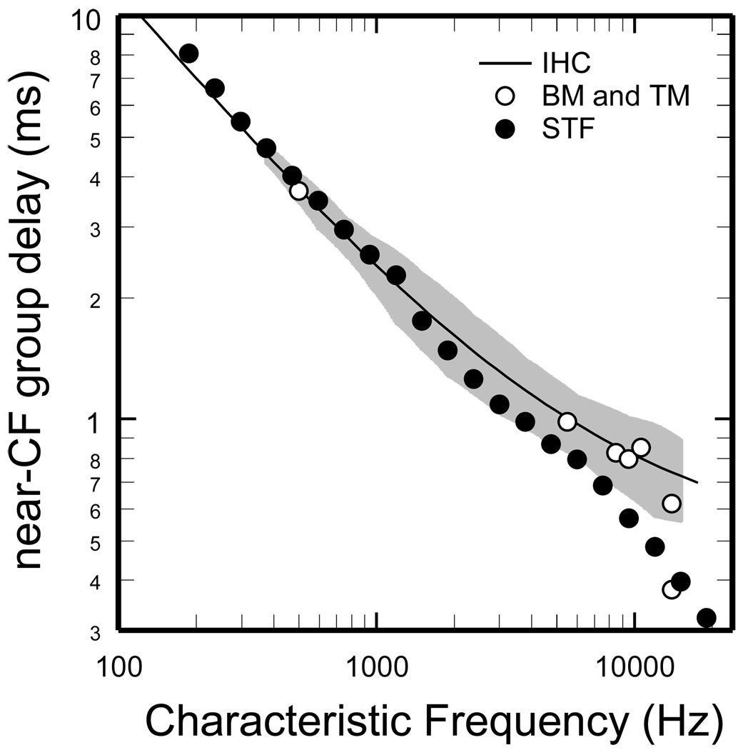
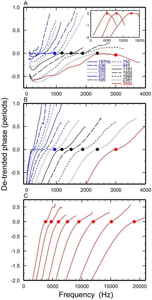
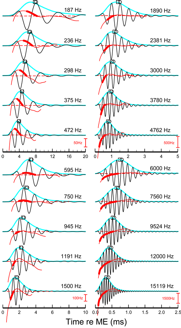
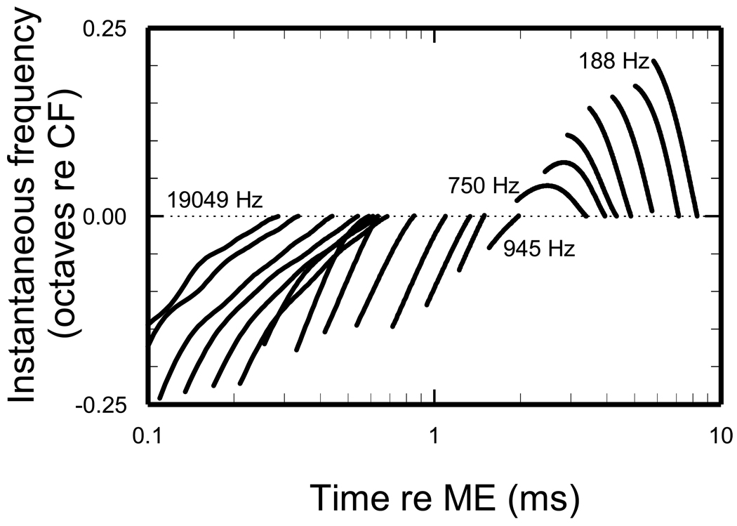
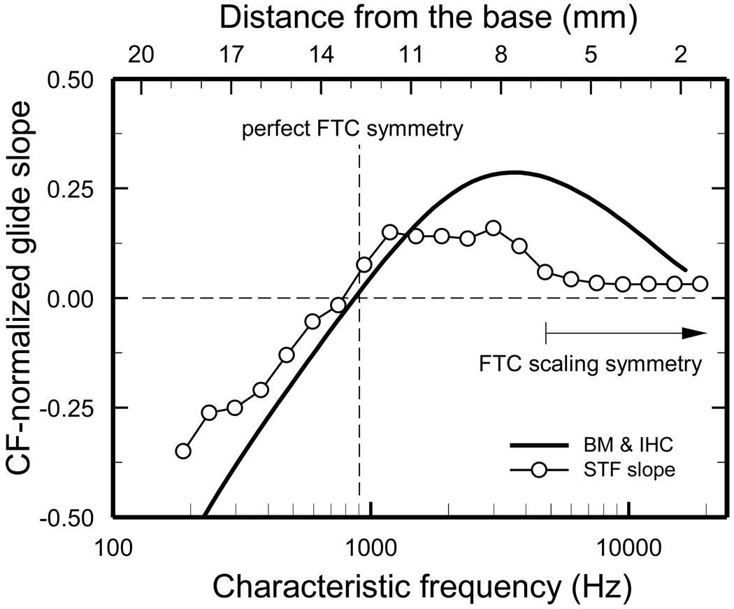
Links between frequency tuning and timing were explored in the responses to sound of auditory-nerve fibers. Synthetic transfer functions were constructed by combining filter functions, derived via minimum-phase computations from average frequency-threshold tuning curves of chinchilla auditory-nerve fibers with high spontaneous activity (Temchin et al., 2008), and signal-front delays specified by the latencies of basilar-membrane and auditory-nerve fiber responses to intense clicks (Temchin et al., 2005). The transfer functions predict several features of the phase-frequency curves of cochlear responses to tones, including their shape transitions in the regions with characteristic frequencies of 1 kHz and 3-4 kHz (Temchin and Ruggero, 2010). The transfer functions also predict the shapes of cochlear impulse responses, including the polarities of their frequency sweeps and their transition at characteristic frequencies around 1 kHz. Predictions are especially accurate for characteristic frequencies <1 kHz.

Figure 1. BM velocity gains and tuning curve compared with an average ANF FTC for a site of the chinchilla cochlea with CF of 9.5 kHz

A) Connected open symbols indicate BM velocities for responses to tones presented at 0–100 dB SPL, in steps of 10 dB. The red flat line indicates a velocity magnitude of 132 µm/s. The red filled symbols indicate stimulus frequency/level combinations that elicit 132 µm/s, the BM velocity at 12.3 dB SPL (the CF threshold of the average FTC for high-spontaneous-rate ANFs with CF = 9.5 kHz). B) Connected open symbols indicate the same BM responses of panel A after normalization to SPL. The red filled symbols indicate a BM tuning curve, plotted relative to level at CF, for a 132-µm/s velocity magnitude. The solid red trace indicates an average FTC (scale to right), for ANFs with high spontaneous activity. BM data from (Ruggero et al., 2000). The dashed red line indicates an extrapolation and truncation of the FTC. ANF data from (Temchin et al., 2008).

Figure 2. Computation of STFs

A) Thick trace: average FTC [from Fig. 4 of (Temchin et al., 2008)] plotted relative to threshold at CF. Thin trace: filter function obtained by extrapolation of the synthetic FTC. B) BM signal-front delays plotted against CF. Trace: trend line for BM signal-front delays, directly measured and/or derived from ANF responses to intense clicks [from Fig. 13A of (Temchin et al., 2005)]. Grey area indicates means +/− standard deviations for BM signal-front delays derived from chinchilla ANF responses to clicks [Fig. 10A of (Temchin et al., 2005)]. C) Thin trace: minimum-phase impulse response derived (see text and Methods) from the filter function of panel A. Thick trace: STF impulse response, obtained by delaying the zero-delay minimum-phase impulse response by 24 µs. D) Thin trace: phase-frequency curve of the minimum-phase filter. Thick trace: phase-frequency curve of the STF. Symbols indicate phase at CF.

Figure 3. Phase-frequency functions of minimum-phase filters

A) CFs ≤ 3 kHz. B) CFs ≥ 3.78 kHz. Open symbols indicate phase at CF. Filled symbols in panel B represent the phases at CF for CFs ≤ 3 kHz, reproduced from panel A.

Figure 4. Phase-frequency functions of STFs and of measured cochlear responses for CFs ≤ 3 kHz

A) Traces: phase-frequency curves of STFs. Symbols: phase at CF. B) Traces: putative BM phase-frequency curves derived from responses to tones of chinchilla ANFs [modified from Fig. 10A of (Temchin and Ruggero, 2010)]. Open symbols: phase at CF. Filled symbols: phases of tectorial-membrane vibrations at an apical site of the chinchilla cochlea [from Fig. 2B of (Rhode and Cooper, 1996).

Figure 5. Phase-frequency functions of STFs and of measured cochlear responses for CFs > 3.78 kHz

A) Traces: phase-frequency curves of STFs. Symbols: phase at CF. B) Phase-frequency curves for BM responses to tones or clicks measured in many chinchilla cochleae [Fig. 5B of (Rhode and Recio, 2000), Fig. 1D of (Rhode, 2007), Fig. 13 of (Ruggero et al., 1997), Fig. 1C of (Ruggero et al., 1997), Fig. 2 of (Narayan and Ruggero, 2000), Fig. 5B of (Rhode and Recio, 2000), Fig. 6A, 6B and 9A of (Recio and Rhode, 2000)]. In some cases CFs are indicated by more than one symbol because different CFs are given in the original publications: 6, 7, 7.9, 10.7, 12.1, 14.3 and 14.7 in (Rhode and Recio, 2000) and 6.1 (or 6.5), 7.1, 9.3, 10.5, 11.7, 12.7 and 13.7 in p. 2286 and Fig. 9A of (Recio and Rhode, 2000).

Figure 6. Near-CF group delays of STFs and of measured cochlear responses

Filled symbols: near-CF group delays of the STFs. Trace: trend line for near-CF group delays of cochlear vibrations [from Figs.11A and 13B of (Temchin et al., 2005)], measured at the BM or tectorial membrane or derived from Wiener kernels of ANF responses to noise presented at near-threshold levels. Open symbols: near-CF group delays of measured BM or tectorial-membrane responses. Grey area indicates means plus/minus standard deviation of near-CF group delays computed from data of Fig. 10B of (Temchin et al., 2005).

Figure 7. De-trended phase-frequency curves of STFs and cochlear vibrations

De-trending consisted of rotating the curves counterclockwise in proportion to group delays at CF. A) De-trended phase-frequency curves of putative IHCs, derived from ANF responses [Fig. 11 of (Temchin and Ruggero, 2010)]. Inset: similarly de-trended phase-frequency curves for BM responses at basal sites of the chinchilla cochlea. Symbols mark de-trended phase at CF. BM data from Fig. 1C of (Ruggero et al., 2000), Fig. 5 of (Recio and Rhode, 2000), and Fig. 2 of (Narayan and Ruggero, 2000). B) De-trended phase-frequency curves of STFs for CFs ≤ 3 kHz. Legend in panel A also applies. C) De-trended phase-frequency curves of STFs for CFs ≥ 3.78 kHz.

Figure 8. STF impulse responses

Each STF impulse response was computed as exemplified in Fig. 2. The STF CFs (in 1/3-octaves steps) span most of the length of the chinchilla cochlea. Squares: weighted-average group delays. Circles: near-CF group delays (same as filled symbols in Fig. 6). Blue traces: magnitudes of the STF impulse-response envelopes. Red traces indicate instantaneous frequencies at times corresponding to response envelope magnitudes exceeding 10% of maximum. Thick red trace indicates the segment of the instantaneous-frequency curve between the first trough of the STF and CF. Dashed red lines indicate CF. Frequency scales (red) apply to the 5 traces immediately above it.

Figure 9. Frequency glides of STF impulse responses

Thick trace indicates the segment of the instantaneous-frequency curve between the first trough of the STF impulse response and CF (i.e., thick red traces in Fig. 8), plotted as functions of time for CFs spaced at 1/3-octave intervals.

Figure 10. Instantaneous-frequency slopes of STF and measured cochlear impulse responses

Open circles: slopes of the STF frequency glides, computed from the first STF trough and CF (spans indicated by thick traces in Figs. 8 and 9). Solid trace: average dimensionless slopes of frequency glides in BM responses to clicks and putative IHC impulse responses derived from Wiener kernels of chinchilla ANF responses to noise [Fig. 17C of (Recio-Spinoso et al., 2005)]. The vertical dashed line indicates the CF (~900 Hz) about which ANF FTCs are symmetrical [Figs.5 of (Temchin et al., 2008) and 3 of (Temchin and Ruggero, 2010)]. The horizontal arrow labeled “FTC scaling symmetry” indicates the (basal) region of the chinchilla cochlea (CFs ≥ 4.8 kHz) in which ANF FTCs plotted with abscissa representing log(frequency/CF) are identical [Fig. 7C of (Temchin et al., 2008)], indicating that the envelopes of the traveling wave are also identical (Zweig, 1976)]. The distance scale was computed from CFs according to the cochlear map of (Müller et al., 2010).

References

1. Bode HW. Network Analysis and Feedback Amplifier Design. New York: 1945.
1. de Boer E, Nuttall AL. The mechanical waveform of the basilar membrane. I. Frequency modulations ("glides") in impulse responses and cross-correlation functions. J Acoust Soc Am. 1997;101:3583–3592. - PubMed
1. Goldstein JL, Baer T, Kiang NY. A theoretical treatment of latency, group delay and tuning. Characteristics for auditory nerve responses to clicks and tones. In: Sachs MB, editor. The Physiology of the Auditory System. Baltimore: National Educational Consultants; 1971. pp. 133–141.
1. Huang S, Dong W, Olson EC. Subharmonics and auditory nerve tuning curves. Assoc.Res.Otolaryngol., Midwinter Meet. Abstracts. 2010;33:255.
1. IEEE. Programs for Digital Signal Processing. New York: IEEE Press; 1979.
Publication types