. 2010 Nov 21;55(22):6575-99.
doi: 10.1088/0031-9155/55/22/001. Epub 2010 Oct 20.

Evaluation of sparse-view reconstruction from flat-panel-detector cone-beam CT

Affiliations

Evaluation of sparse-view reconstruction from flat-panel-detector cone-beam CT

Junguo Bian et al. Phys Med Biol. .

Abstract

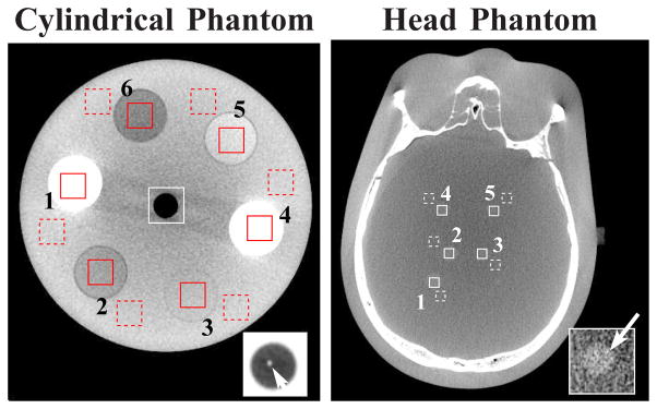
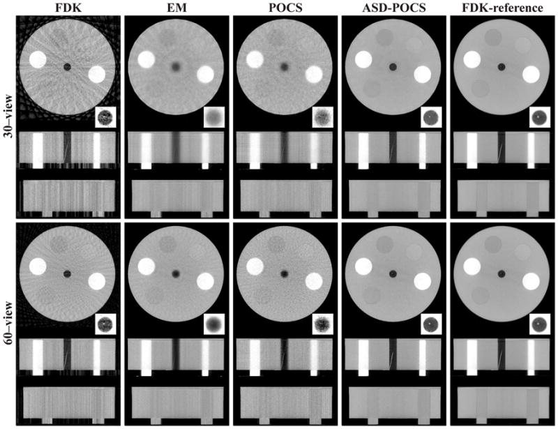
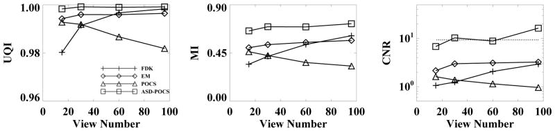
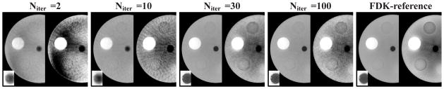
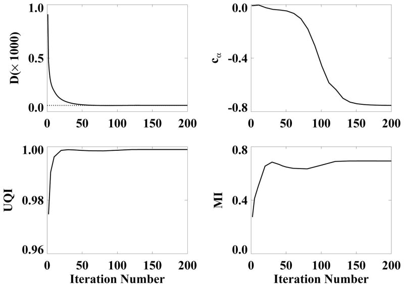
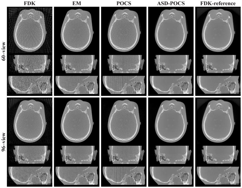
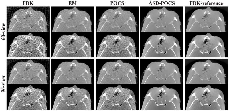
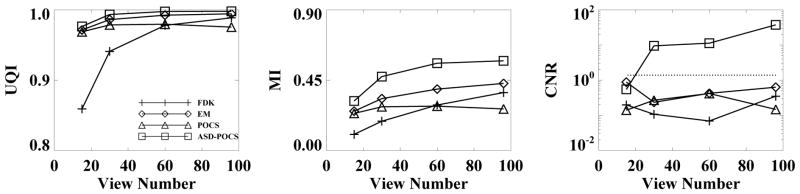
Flat-panel-detector x-ray cone-beam computed tomography (CBCT) is used in a rapidly increasing host of imaging applications, including image-guided surgery and radiotherapy. The purpose of the work is to investigate and evaluate image reconstruction from data collected at projection views significantly fewer than what is used in current CBCT imaging. Specifically, we carried out imaging experiments using a bench-top CBCT system that was designed to mimic imaging conditions in image-guided surgery and radiotherapy; we applied an image reconstruction algorithm based on constrained total-variation (TV)-minimization to data acquired with sparsely sampled view-angles and conducted extensive evaluation of algorithm performance. Results of the evaluation studies demonstrate that, depending upon scanning conditions and imaging tasks, algorithms based on constrained TV-minimization can reconstruct images of potential utility from a small fraction of the data used in typical, current CBCT applications. A practical implication of the study is that the optimization of algorithm design and implementation can be exploited for considerably reducing imaging effort and radiation dose in CBCT.


Figures

Figure 1
Figure 1
Images of the cylindrical and head phantoms within a transverse slice at z = 0 cm reconstructed from full data by use of the FDK (row 1) and ASD-POCS (row 2) algorithms. For the cylindrical-phantom, the entire images are displayed with a wide (i.e., bone-grayscale) window [−1000, 714] HU; rectangle regions enclosed by dashed lines (i.e., ROIs 1 and 2) are redisplayed in the upper-left and lower-left corners with a narrow (i.e., soft-tissue-grayscale) window [−257, 143] HU; and the rectangle region enclosed by solid lines (i.e., ROI 3) is re-displayed in the lower-right corner with a zoomed-in view in a grayscale window of [−1000, −143] HU, with an arrow pointing to a wire insert. For the head phantom, the entire images are displayed with a wide bone-grayscale window [−1000, 1000] HU; ROIs 1 and 2 are re-displayed in the upper-left and lower-left corners with a narrow window [−429, 429] HU; ROI 3 is re-displayed in the lower-right corner by use of a zoomed-in view with the bone-grayscale window.
Figure 2
Figure 2
s-ROIs (solid-line squares) and b-ROIs (dashed-line squares) selected within transverse slices at z = 2.0 cm in the cylindrical phantom (left) and z = 1.2 cm in the head phantom (right) for CNR computation. The ROIs in cylindrical phantom correspond to cortical bone (ROI 1 and ROI 4) and breast (ROI 2), brain (ROI 3), liver (ROI 5) and adipose (ROI 6) tissues. The cylindrical and head phantom images are displayed with soft-tissue-grayscale windows of [−257, 143] HU and [−429, 429] HU. The wire insert in the central region of the cylindrical phantom and ROI 2 of the head phantom, which are displayed with a zoomed-in view using grayscale windows of [−1000, −143] HU and [−200, 28] HU, are used as the signals for the detectability calculation. Cupping artifacts can be observed as a result of physical factors, such as beam-hardening and scatter, when the image is displayed with a narrow grayscale window.
Figure 3
Figure 3
Images of the cylindrical phantom reconstructed from 30-view (rows 1–3) and 60-view (rows 4–6) data sets by use of the FDK, EM, POCS, and ASD-POCS algorithms, within a transverse slice at z = 2.0 cm (rows 1 and 4), coronal slice at x = −3.0 cm (rows 2 and 5), and sagittal slice at y = −0.25 cm (rows 3 and 6). The central region of the transverse slice is redisplayed with a zoomed-in view using a grayscale window of[−1000, −143] HU to show the wire insert. The last column is the FDK-reference images within the corresponding slices. A bone grayscale window, [−1000, 714] HU, is used.
Figure 4
Figure 4
Images of the cylindrical phantom reconstructed from 30-view (rows 1–3) and 60-view (rows 4–6) data sets by use of the FDK, EM, POCS, and ASD-POCS algorithms, within a transverse slice at z = 2.0 cm (rows 1 and 4), coronal slice at x = −3.0 cm (rows 2 and 5), and sagittal slice at y = −0.25 cm (rows 3 and 6). The central region of the transverse slice is redisplayed with a zoomed-in view using a grayscale window of [−571, −429] HU to show the wire insert. The last column is the FDK-reference images within the corresponding slices. A soft-tissue grayscale window, [−257, 143] HU, is used.
Figure 5
Figure 5
UQI (left), MI (middle), and CNR (right) as functions of projection views, computed from the cylindrical phantom images reconstructed by use of the FDK (+), EM (◇), POCS (△), and ASD-POCS (□) algorithms and the FDK-reference image. The dotted line displays the corresponding CNR in the FDK-reference image.
Figure 6
Figure 6
ROI images of the cylindrical phantom within a transverse slice at z = 0 cm reconstructed from 60-view data by use of the ASD-POCS algorithm at iterations 2, 10, 30, and 100. For each displayed iteration number, the ROI image are shown with a bone-grayscale window [−1000, 714] HU (left) and a soft-tissue-grayscale window [−257, 143] HU (right). The square ROI shows the zoomed-in view of the central region containing the wire with a grayscale window [−1000, −143] HU.
Figure 7
Figure 7
Image-property parameters, as functions of iteration numbers for images reconstructed from 60-view data by use of the ASD-POCS algorithm. Row 1: data divergence D (left) and parameter cα (right); and row 2: UQI (left) and MI (right) calculated within the entire image support. The dotted line in data-divergence plot indicates the selected ε.
Figure 8
Figure 8
Power spectra of the cylindrical phantom obtained from 15-, 30-, 60-, and 96-view data sets by use of the FDK (+), EM (◇), POCS (△), and ASD-POCS (□) algorithms. The power spectrum of the FDK-reference image is plotted as the dotted curve.
Figure 9
Figure 9
Detectabilities for the wire as functions of projection views (left) and iteration number (right) calculated from cylindrical phantom images reconstructed by use of the FDK (+), EM (◇), POCS (△), and ASD-POCS (□) algorithms. The detectability of the FDK-reference image is plotted as dotted lines.
Figure 10
Figure 10
Images of the head phantom reconstructed from 60-view (rows 1–3) and 96-view (rows 4–6) data sets by use of the FDK, EM, POCS, and ASD-POCS algorithms, within a transverse slice at z = 1.2 cm (rows 1 and 4), coronal slice at x = 0.6 cm (rows 2 and 5), and, sagittal slice at y = 2.5 cm (rows 3 and 6). The last column displays the FDK-reference images within the corresponding slices. A bone grayscale window, [−1000, 1000] HU, is used.
Figure 11
Figure 11
Images of the head phantom reconstructed from 60-view (rows 1–3) and 96-view (rows 4–6) data sets by use of the FDK, EM, POCS, and ASD-POCS algorithms, within a transverse slice at z = 1.2 cm (rows 1 and 4), coronal slice at x = 0.6 cm (rows 2 and 5), and sagittal slice at y = 2.5 cm (rows 3 and 6). The last column displays the FDK-reference images within the corresponding slices. A soft-tissue grayscale window, [−429, 429] HU, is used. Low-contrast tumor structures can be observed in the ASD-POCS reconstructions and FDK-reference images.
Figure 12
Figure 12
Nasal-region images of the head phantom within a transverse slice at z = 0 cm reconstructed from 60-view (row 1–2) and 96-view (row 3–4) data sets by use of the FDK, EM, POCS, and ASD-POCS algorithms displayed in a bone grayscale window of [−1000, 1000] HU (row 1 and 3) and a soft-tissue grayscale window of [−429, 429] HU (row 2 and 4). The corresponding FDK-reference images are shown in the last column.
Figure 13
Figure 13
UQI (left), MI (middle) and CNR (right) as functions of projection views, computed from the head phantom images reconstructed by use of the FDK (+), EM (◇), POCS (△), and ASD-POCS (□) algorithms and the FDK-reference image. The dotted line displays the corresponding CNR in the FDK-reference image.
Figure 14
Figure 14
Nasal-region images of the head phantom within a transverse slice at z = 0 cm reconstructed from 96-view data by use of the ASD-POCS algorithm at iterations 2, 10, 30, and 100, displayed with a bone-grayscale window [−1000, 1000] HU (row 1) and a soft-tissue grayscale window [−429, 429] HU (row 2).
Figure 15
Figure 15
Power spectra of the head phantom obtained from 15-, 30-, 60-, and 96-view data sets by use of the FDK (+), EM (◇), POCS (△), and ASD-POCS (□) algorithms. The power spectrum of the FDK-reference image is plotted as the dotted curve.
Figure 16
Figure 16
Detectabilities for the low-contrast lesions as functions of projection views (left) and iteration number (right) calculated from head phantom images reconstructed by use of the FDK (+), EM (◇), POCS (△;), and ASD-POCS (□) algorithms. The detectability of the FDK-reference image is plotted as dotted lines.
Figure 17
Figure 17
Profiles along two lines within the transverse slice at z = 0 cm in the FDK- (dotted curve) and ASD-POCS-reference (solid curve) images and in the 60-view, ASD-POCS reconstruction (dashed curve) of the cylindrical phantom. It is obvious that the images are not piece-wise constant.
Figure 18
Figure 18
Row 1: Power spectra computed from the FDK-reference (dotted curve) and ASD-POCS-reference (solid curve) images. Row 2: MIs, as functions of projection views, computed from cylindrical (left) and head (right) phantom images obtained by use of the FDK (+), EM (◇), POCS (△), and ASD-POCS (□) algorithms and the ASD-POCS-reference image. They differ from their counterparts in Figs. 5 and 13, which were obtained with the FDK-reference images.

Similar articles

Cited by

References

    1. Brenner DJ, Hall EJ. Computed tomography–an increasing source of radiation exposure. N Engl J Med. 2007;357:2277–2284. - PubMed
    1. De Gonzalez AB, Mahesh M, Kim K, Bhargavan M, Lewis R, Mettler F, Land C. Projected cancer risks from computed tomographic scans performed in the United States in 2007. Arch Intern Med. 2009;169:2071–2077. - PMC - PubMed
    1. Smith-Bindman R, Lipson J, Marcus R, Kim K, Mahesh M, Gould R, de Gonzalez AB, Miglioretti DL. Radiation dose associated with common computed tomography examinations and the associated lifetime attributable risk of cancer. Arch Intern Med. 2009;169:2078–2086. - PMC - PubMed
    1. Feldkamp LA, Davis LC, Kress JW. Practical cone-beam algorithm. J Opt Soc Am A. 1984;1:612–619.
    1. Katsevich A. Theoretically exact filtered backprojection-type inversion algorithm for spiral CT. SIAM J Appl Math. 2002;62:2012–2026.

Publication types

MeSH terms