

The statistical mechanics of a polygenic character under stabilizing selection, mutation and drift
- PMID: 21084341
- PMCID: PMC3061091
- DOI: 10.1098/rsif.2010.0438
The statistical mechanics of a polygenic character under stabilizing selection, mutation and drift
Abstract
By exploiting an analogy between population genetics and statistical mechanics, we study the evolution of a polygenic trait under stabilizing selection, mutation and genetic drift. This requires us to track only four macroscopic variables, instead of the distribution of all the allele frequencies that influence the trait. These macroscopic variables are the expectations of: the trait mean and its square, the genetic variance, and of a measure of heterozygosity, and are derived from a generating function that is in turn derived by maximizing an entropy measure. These four macroscopics are enough to accurately describe the dynamics of the trait mean and of its genetic variance (and in principle of any other quantity). Unlike previous approaches that were based on an infinite series of moments or cumulants, which had to be truncated arbitrarily, our calculations provide a well-defined approximation procedure. We apply the framework to abrupt and gradual changes in the optimum, as well as to changes in the strength of stabilizing selection. Our approximations are surprisingly accurate, even for systems with as few as five loci. We find that when the effects of drift are included, the expected genetic variance is hardly altered by directional selection, even though it fluctuates in any particular instance. We also find hysteresis, showing that even after averaging over the microscopic variables, the macroscopic trajectories retain a memory of the underlying genetic states.
Figures


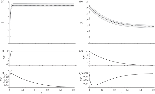
 , 〈ν〉 = 1.12. Dashed line: Nβ = 0
  . Dotted line: Nβ = −2.5,
  ,
,  . (b) Changing the intensity of selection over the genetic variance modulates the position of the adaptive peaks (other things being equal, Nβ = 2.5), resulting in pronounced changes in the expectation of the genetic variance, but with weak changes on the expectation of the trait mean. Dotted line: Nσ = 0,
  , 〈ν〉 = 8.04. Short-dashed line: Nσ = −1,
  ,
,  . Large-dashed line: Nσ =− 4,
  ,
,  . Solid line: Nσ = −10,
  ,
,  . In all cases Nμ = 0.5, Nλ = −1.0, and the trait is composed of 20 loci of equal effects.


Similar articles
-
A General Approximation for the Dynamics of Quantitative Traits.Genetics. 2016 Apr;202(4):1523-48. doi: 10.1534/genetics.115.184127. Epub 2016 Feb 17. Genetics. 2016. PMID: 26888079 Free PMC article.
-
Statistical mechanics and the evolution of polygenic quantitative traits.Genetics. 2009 Mar;181(3):997-1011. doi: 10.1534/genetics.108.099309. Epub 2008 Dec 15. Genetics. 2009. PMID: 19087953 Free PMC article.
-
Polygenic dynamics underlying the response of quantitative traits to directional selection.Theor Popul Biol. 2024 Aug;158:21-59. doi: 10.1016/j.tpb.2024.04.006. Epub 2024 Apr 26. Theor Popul Biol. 2024. PMID: 38677378
-
Clines in polygenic traits.Genet Res. 1999 Dec;74(3):223-36. doi: 10.1017/s001667239900422x. Genet Res. 1999. PMID: 10689800 Review.
-
Polygenic Adaptation in a Population of Finite Size.Entropy (Basel). 2020 Aug 18;22(8):907. doi: 10.3390/e22080907. Entropy (Basel). 2020. PMID: 33286676 Free PMC article. Review.
Cited by
-
Adaptive fixation in two-locus models of stabilizing selection and genetic drift.Genetics. 2014 Oct;198(2):685-97. doi: 10.1534/genetics.114.168567. Epub 2014 Aug 4. Genetics. 2014. PMID: 25091496 Free PMC article.
-
A Genomic Map of the Effects of Linked Selection in Drosophila.PLoS Genet. 2016 Aug 18;12(8):e1006130. doi: 10.1371/journal.pgen.1006130. eCollection 2016 Aug. PLoS Genet. 2016. PMID: 27536991 Free PMC article.
-
Dynamic maximum entropy provides accurate approximation of structured population dynamics.PLoS Comput Biol. 2021 Dec 1;17(12):e1009661. doi: 10.1371/journal.pcbi.1009661. eCollection 2021 Dec. PLoS Comput Biol. 2021. PMID: 34851948 Free PMC article.
-
A General Approximation for the Dynamics of Quantitative Traits.Genetics. 2016 Apr;202(4):1523-48. doi: 10.1534/genetics.115.184127. Epub 2016 Feb 17. Genetics. 2016. PMID: 26888079 Free PMC article.
-
Stability and response of polygenic traits to stabilizing selection and mutation.Genetics. 2014 Jun;197(2):749-67. doi: 10.1534/genetics.113.159111. Epub 2014 Apr 7. Genetics. 2014. PMID: 24709633 Free PMC article.
References
-
- Lande R. 1979. Quantitative genetic analysis of multivariate evolution, applied to brain: body size allometry. Evolution 33, 402–41610.2307/2407630 (doi:10.2307/2407630) - DOI - DOI - PubMed
-
- Turelli M. 1988. Phenotypic evolution, constant covariances, and the maintenance of additive variance. Evolution 42, 1342–134710.2307/2409017 (doi:10.2307/2409017) - DOI - DOI - PubMed
-
- Lynch M., Walsh B. 1998. Genetics and analysis of quantitative traits. Sunderland, MA: Sinauer Associates
-
- Barton N. H., Turelli M. 1987. Adaptive landscapes, genetic distance and the evolution of quantitative characters. Genet. Res. 49, 157–17310.1017/S0016672300026951 (doi:10.1017/S0016672300026951) - DOI - DOI - PubMed
-
- Bürger R. 2000. The mathematical theory of selection, recombination and mutation. Oxford, UK: Wiley & Son
Publication types
MeSH terms
Grants and funding
LinkOut - more resources
Full Text Sources
