The importance of structured noise in the generation of self-organizing tissue patterns through contact-mediated cell-cell signalling

Abstract

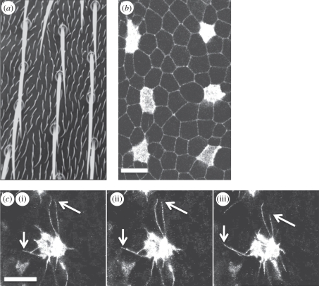
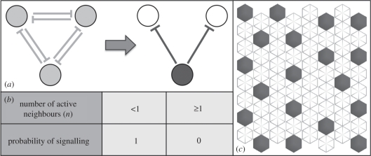
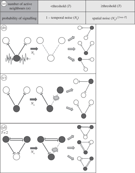
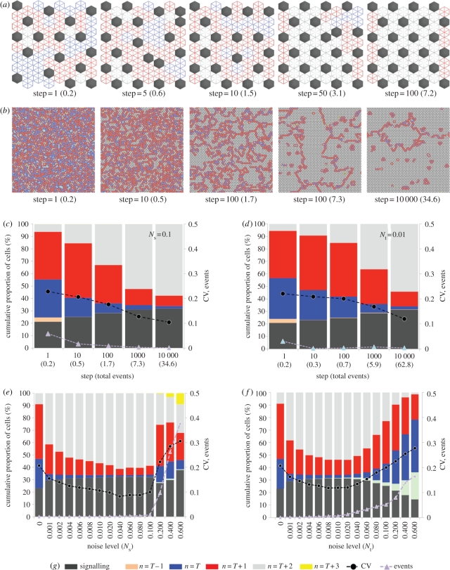
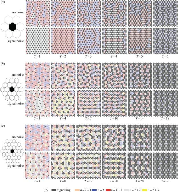
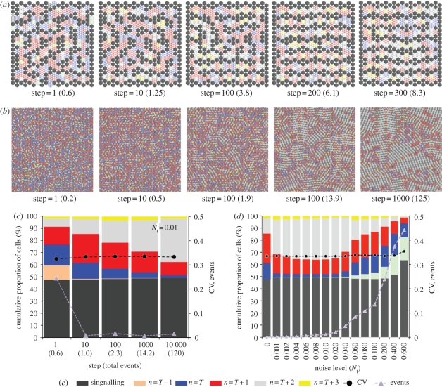
Lateral inhibition provides the basis for a self-organizing patterning system in which distinct cell states emerge from an otherwise uniform field of cells. The development of the microchaete bristle pattern on the notum of the fruitfly, Drosophila melanogaster, has long served as a popular model of this process. We recently showed that this bristle pattern depends upon a population of dynamic, basal actin-based filopodia, which span multiple cell diameters. These protrusions establish transient signalling contacts between non-neighbouring cells, generating a type of structured noise that helps to yield a well-ordered and spaced pattern of bristles. Here, we develop a general model of protrusion-based patterning to analyse the role of noise in this process. Using a simple asynchronous cellular automata rule-based model we show that this type of structured noise drives the gradual refinement of lateral inhibition-mediated patterning, as the system moves towards a stable configuration in which cells expressing the inhibitory signal are near-optimally packed. By analysing the effects of introducing thresholds required for signal detection in this model of lateral inhibition, our study shows how filopodia-mediated cell-cell communication can generate complex patterns of spots and stripes, which, in the presence of signalling noise, align themselves across a patterning field. Thus, intermittent protrusion-based signalling has the potential to yield robust self-organizing tissue-wide patterns without the need to invoke diffusion-mediated signalling.

Figure 1.

Sensory organ patterning is driven by signalling between dynamic cellular protrusions. (a) A section of the notum of an adult Drosophila melanogaster fruitfly displays the evenly spaced, grid-like pattern of microchaete bristles that act as mechanosensory organs. Between each bristle are ordinary epithelial cells, each of which expresses a small hair. (b) The development of the pattern of mechanosensory organ precursor cells can be observed in fly pupae. The image shows the apical section of epithelial cells in an area of the notum close to the fly midline, at 14 h after pupae formation. Cells destined to become sensory organs (microchaete bristles) express Neuralized-Gal4, UAS-Moesin-GFP (Neu-GFP). Ubiquitously expressed E-Cadherin-GFP is used to visualize apical cell–cell junctions. (c) Confocal sections reveal the dynamic protrusions (filopodia and lamelopodia) in the basal section of a typical epithelial cell. The cell in this example is imaged through its expression of Neu-GFP. The image shows the position of filopodia at three 100 s intervals, which extend over multiple cell diameters. The arrows highlight the ends of two filopodia that can be observed extending and retracting (mean filopodia lifetime approx. 500 s—data not shown). Scale bars, 10 µm, (c) (i) 0 s, (ii) 100 s, (iii) 200 s.

Figure 2.

Simulating lateral inhibition patterning. (a) A schematic of the lateral inhibition patterning. Initially homogeneous cells (light grey) compete to express an inhibitory signal. Eventually a single cell becomes active (dark grey) and strongly inhibits the expression of the signal in its contacting neighbours. (b) The outcome of lateral inhibition signalling expressed as a probabilistic rule set. The signalling probability determines whether a single cell in a field will express an inhibitory signal based on the total number of its active signalling neighbours (n). (c) An asynchronous cellular automata simulation of lateral inhibition. Cells in the 8 × 8 hexagonally packed array are sequentially selected at random and updated according to the rule table in (b). The outcome is a notably disordered packing of active cells (dark grey) expressing the inhibitory signal.

Figure 3.

An enhanced model of lateral inhibition incorporating signalling noise and different inhibitory thresholds. (a) The rule table determines the probability that a selected cell in an asynchronous cellular automaton will actively express an inhibitory signal. The threshold (T) is the minimum number of active signalling cells (n) required to inhibit an inactive cell. Temporal noise (N_t) is the probability that a cell will stop signalling even without an inhibitory signal at the required threshold. Spatial noise(N_s) is the probability that an inactive cell will signal even when it is in contact with the threshold number of active signalling cells. This probability reduces as the number of active neighbours increases over the threshold. (b) A schematic of pattern shifting owing to temporal signalling noise. A cell's inhibitory signal (dark grey) oscillates over time. Its signal effectively ceases such that at subsequent time steps neighbouring cells that were previously inhibited may become active. (c) A schematic of pattern shifting owing to spatial signalling noise. A signal ‘connection’ is broken and an inactive cell (white) no longer receives an inhibitory signal and becomes active. At subsequent time steps when the connection is re-established, the cells compete and a stable configuration is re-established. (d) A representation of spatial noise in which a minimum threshold of two active cells is required to inhibit a third cell. As in (c) the pattern may shift as a result of the signal noise.

Figure 4.

Signal noise leads to pattern optimization. (a,b) Simulations of inhibitory signalling with spatial noise, N_s = 0.1, T = 1, (a) executed in an 8 × 8 hexagonally packed array of cells and (b) a 100 × 100 array of cells with toroidal boundaries. Each image shows the pattern at a particular ‘step’ in the simulation advancing from left to right. A single step represents a number of cell updates equal to the total number of cells in the array. The number shown in brackets represents the total proportion of cells that have switched state (total events). The state of cells is defined by the colour key in (g): dark-grey cells actively express the inhibitory signal and all inactive cells are coloured according to their total number of active neighbours. As the patterns move towards a state of optimized packing this corresponds to a reduction in the number of blue (one active neighbour) and red (two active neighbours) cells and an increase in the number of light-grey cells (three active neighbours). Note that with spatial noise adjacent cells sometimes signal (see steps 5 and 50 in (a)), which causes the shift in the pattern towards the optimized state (compare with optimization under temporal noise in the electronic supplementary material, figure S1). In a large field (b) this leads to the development of relatively stable optimized ‘zones’ with unstable active boundaries, which expand over time. See also the electronic supplementary material, movie 1. (c,d) The change over time in the proportion of each cell type represented as a cumulative percentage (plotted on the left-hand y-axis). Data are averaged over 10 simulations. In (c) the conditions are as described in (b). The results of identical simulations with temporal noise, N_t = 0.01 are shown in (d). In addition, the purple triangles show the number of events occurring at each step. The black circles show the coefficient of variation (CV) in the pattern spacing that was measured by recording the distance between each active cell and its six nearest neighbours and taking the ratio of the standard deviation to the mean. The CV and events are plotted on the right-hand y-axis. (e,f) A comparison of the final pattern state achieved after 10 000 steps with different amounts of spatial noise (e) and temporal noise (f). The figures show the mean values from 10 simulations. Optimized patterns are achieved with noise levels in the ranges 0.001 < N_s < 0.1 and 0.001 < N_t < 0.01. At higher levels of noise, the patterns become unstable, as represented by the significant increase in the number of events. NB: Standard errors (95% confidence intervals) in the mean data displayed in (c–f) were less than 1% (left-hand y-axis) and less than 0.01 (right-hand y-axis) and so were not visible on this scale.

Figure 5.

At different signal ranges and inhibitory thresholds, a broad scope of patterns can be achieved. (a–c) Each panel shows typical results after 1000 steps for simulations of inhibitory signalling carried out in a 20 × 20 hexagonally packed array of cells. Different signal ranges were implemented, as illustrated by the size of the hexagonal shells positioned on the left ((a) one cell, (b) two cells and (c) three cells). For each signal range, a selection of inhibitory thresholds is shown with and without temporal noise, N_t = 0.01. The active signalling cells and the neighbourhood of inactive cells are identified according to the key in (d). It is clear from this illustrative set of examples that different patterns are achievable ranging from spots through to stripes that may be in some cases realigned by the input of signal noise (e.g. (b), T = 10).

Figure 6.

Patterns of stripes align owing to signal noise. (a,b) Simulations of inhibitory signalling with a signalling range of two cells, an inhibitory threshold, T = 9, and temporal signalling noise, N_t = 0.01. The active signalling cells and the neighbourhood of inactive cells are labelled according to the colour key in (e). The number of simulations steps and total events (in brackets) is shown progressing from left to right. In (a), where a small array of 20 × 20 cells was used, the initial pattern of randomly orientated stripes can be seen to align, over time, with the array boundaries where there is no signal. In (b), where a larger array of 100 × 100 cells (with toroidal boundaries) was used, distinct zones of aligned stripes are formed as a result of the signalling noise. See also the electronic supplementary material, movie 2. (c) Graphical visualization of the patterning process. The figure shows the cumulative proportion of each cell type (as defined in the colour key in (e)) obtained from data averaged over 10 simulations with the conditions specified in (b). The process of stripe alignment correlates with a transition from n = T and n = T + 1 cells to n = T + 2 cells. Also plotted are the number of events per time step and the CV in the pattern spacing. With stripe alignment there is no change in the CV of the pattern spacing. (d) A comparison of the final pattern state achieved after 10 000 steps with different amounts of signal noise. The figures show the mean values obtained after 10 simulations at a signal range of two cells and a threshold, T = 9. Optimized patterns are achieved with noise levels in the range 0.001 < N_t <0.01. Similar results (data not shown) were obtained when spatial noise was used instead of (or in addition to) temporal noise. NB: Standard errors (95% confidence intervals) in the mean values plotted in (c,d) were less than 1% (left-hand y-axis) and less than 0.01 (right-hand y-axis) and so were not visible on this scale.

References

1. Classen A. K., Anderson K. I., Marois E., Eaton S. 2005. Hexagonal packing of Drosophila wing epithelial cells by the planar cell polarity pathway. Dev. Cell 9, 805–81710.1016/j.devcel.2005.10.016 (doi:10.1016/j.devcel.2005.10.016) - DOI - DOI - PubMed
1. Cohen M., Georgiou M., Stevenson N. L., Miodownik M., Baum B. 2010. Dynamic filopodia drive pattern refinement via intermittent N-Dl signalling. Dev. Cell 19, 78–8910.1016/j.devcel.2010.06.006 (doi:10.1016/j.devcel.2010.06.006) - DOI - DOI - PubMed
1. Maini P. K., Baker R. E., Chuong C.-M. 2006. Developmental biology. The Turing model comes of molecular age. Science 314, 1397–139810.1126/science.1136396 (doi:10.1126/science.1136396) - DOI - DOI - PMC - PubMed
1. Webb S. D., Owen M. R. 2004. Oscillations and patterns in spatially discrete models for developmental ligand-receptor interactions. J. Math. Biol. 48, 444–47610.1007/s00285-003-0247-1 (doi:10.1007/s00285-003-0247-1) - DOI - DOI - PubMed
1. Amoyel M., Cheng Y. C., Jiang Y.-J., Wilkinson D. G. 2005. Wnt1 regulates neurogenesis and mediates lateral inhibition of boundary cell specification in the zebrafish hindbrain. Development 132, 775–78510.1242/dev.01616 (doi:10.1242/dev.01616) - DOI - DOI - PubMed
MeSH terms
LinkOut - more resources