A geometrical model for DNA organization in bacteria

Abstract

Recent experimental studies have revealed that bacteria, such as C. crescentus, show a remarkable spatial ordering of their chromosome. A strong linear correlation has been found between the position of genes on the chromosomal map and their spatial position in the cellular volume. We show that this correlation can be explained by a purely geometrical model. Namely, self-avoidance of DNA, specific positioning of one or few DNA loci (such as origin or terminus) together with the action of DNA compaction proteins (that organize the chromosome into topological domains) are sufficient to get a linear arrangement of the chromosome along the cell axis. We develop a Monte-Carlo method that allows us to test our model numerically and to analyze the dependence of the spatial ordering on various physiologically relevant parameters. We show that the proposed geometrical ordering mechanism is robust and universal (i.e. does not depend on specific bacterial details). The geometrical mechanism should work in all bacteria that have compacted chromosomes with spatially fixed regions. We use our model to make specific and experimentally testable predictions about the spatial arrangement of the chromosome in mutants of C. crescentus and the growth-stage dependent ordering in E. coli.

Figure 1. Representation of DNA as Random Walk.

In the simulations the DNA configuration (black solid line) is represented by a random walk on a three-dimensional cubic lattice. The random walk can be thought of as a discrete set of connected beads. The lattice constant is given by the Kuhn length (which is twice the persistence length ). With this step size the directions of two sequential steps are completely uncorrelated. In the simplest picture the random walk may intersect itself, since the diameter of DNA is much smaller than the grid size.

Figure 2. Average subcellular position of genes as function of their position on the chromosome in C. crescentus as obtained from numerical simulations of non-compacted DNA.

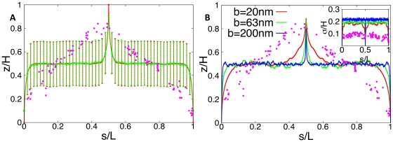
The subcellular position is obtained by averaging the z-positions of 10⁶ different (non self-avoiding) random walks that represent an ensemble of non-compacted chromosomes of C. crescentus confined to the cell volume represented by a lattice of size (corresponding to a volume of for ). The position on the chromosome is parameterized by the contour length s (measured in units of DNA length L). (A) Walk of length 26000b representing the genome. Ori and ter lie on the cell axis at opposite poles. Their distance from the bottom and top cell walls is 0b (red curve) and 4b (green curve). Error bars represent the standard deviations between the different DNA configurations sampled in the 10⁶ runs. Dots represent the experimental data from Ref. . (B) Same plot as in (A) but for different Kuhn lengths (). DNA length and cell volume are kept constant. Here, the standard deviations between the individual realizations are rescaled and shown as function of the position on the chromosome.

Figure 3. Root mean square deviation of the average (non-compacted) DNA configuration from a strictly linear configuration for different DNA lengths and different sizes of the confining volume.

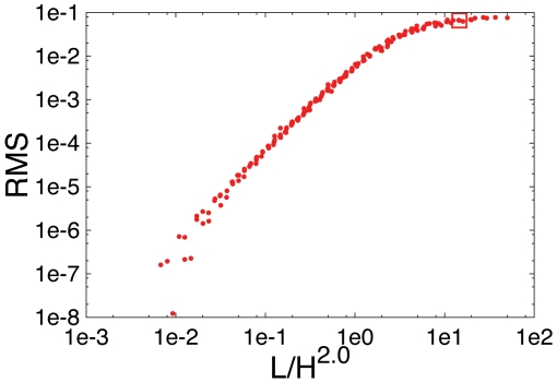
The figure shows the root mean square deviation (RMS) from the strictly linear configuration that connects ori and ter by a line (see Eqs. [1] and [2]) as a function of DNA length L and distance H between ori and ter for cell shapes with the aspect ratio of C. crescentus. RMS is a function of with . The square indicates the data point for L = 26000, H = 40 corresponding to the parameter values of C. crescentus.

Figure 4. Average subcellular position of genes as function of their position on the chromosome in C. crescentus as obtained from numerical simulations of compacted DNA.

The z-position of an average chromosome configuration was calculated from our model in which compacted DNA is represented by a chain of blobs. The position on the chromosome is parameterized by the contour length s (measured in units of DNA length L). The configurations shown are for different blob diameters. In Fig. A a constant density of DNA per blob has been assumed, in Fig. B a constant number (2000) of blobs. The insets show the (rescaled) standard deviations from the mean configurations as function of s. Dots are experimental data from Ref. . The fixed positions of ori and ter (given by and where H is the length of the cell) have been adjusted to minimize the differences between experimental data and the predictions of the model. Figs. C and D are for the same blob parameters as A and B, respectively. However, in C and D only ori has a fixed position at , while ter is free to move. One should note that because of the additional freedom in moving ter the DNA configuration shows a different dependence on the blob size than with fixed ter.

Figure 5. Average DNA configuration in a C. crescentus mutant cell where ori is located at 6 o'clock and ter at 3 o'clock on the chromosome.

In the simulations the chromosome is represented by a self-avoiding chain of blobs with diameter . The chain consists of 2000 blobs: 1500 blobs for the segment connecting ori and ter and 500 blobs for the segment connecting ter and ori. Cell size is . The error bars denote standard deviations from mean position.

Figure 6. Average subcellular position of genes as function of their position on the chromosome in newborn E. coli cells as obtained from numerical simulations of compacted DNA.

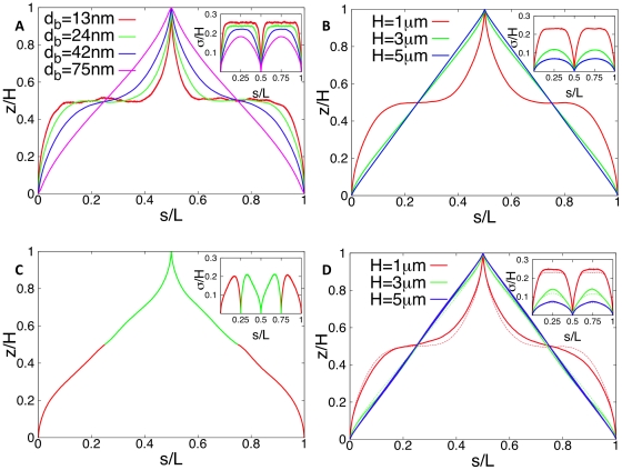
The figure shows the z-position of an average chromosome configuration as function of the contour length s. In our model a chain of blobs represents the compacted DNA. The position on the chromosome is parameterized by s (measured in units of DNA length L). In figures A, B, and D ori and ter are positioned at the cell poles ( and ). The configurations shown in figure A are for a cellular volume of and different blob diameters by assuming a constant density of DNA of per blob. The dependence on the volume at constant DNA density is shown in figure B. Cell shapes are varied at constant cross section but different length (corresponding to H = 33…165 blobs). The largest newborn cell has a volume of . Figure C shows a DNA configuration in a cell with two chromosomes (shown in different colors) just prior to cell division. The two ori have fixed positions at the cell poles, the two ter are kept at midcell. The contour length is measured along the path left (chromosome #1)-right (chromosome #2)-left (chromosome #2)-right (chromosome #1). Data shown are for a volume of and each chromosome is represented by 2000 blobs. In this way the cellular DNA density remains constant and that the length of compacted DNA per blob (given by DNA per blob) is independent of the volume. A DNA configuration in these faster growing cells at an earlier stage of the cell cycle is shown in figure D. Here, the cell contains an additional DNA strand whose ends are anchored in the midplane of the cell mimicking the geometry of the chromosome after half the replication time [when the replication forks are located at 3 o'clock and 9 o'clock on the mother chromosome (solid lines)]. The presence of additional DNA makes the linear correlation stronger. For comparison the DNA configurations without daughter DNA are shown (dashed lines). Parameter values are as in figure B. The insets show the (rescaled) standard deviations from the mean configurations as function of s.

Figure 7. Average subcellular position of genes for different ori and ter positions in E. coli as obtained from numerical simulations of compacted DNA.

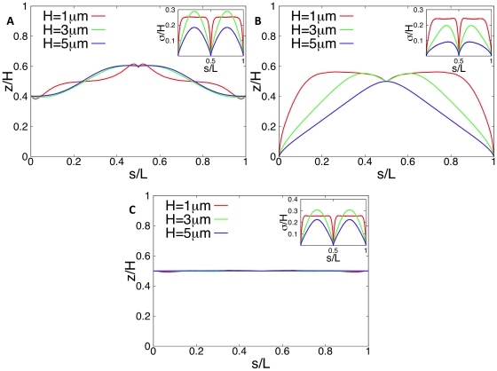
The figures show the z-position of an average chromosome configuration as function of the contour length s. Cell length varies from , i.e. 33 to 165 blob diameters (with a blob diameter of ) at constant DNA density, i.e. the number of blobs is kept constant at 2000. In Fig. A ori and ter are positioned in midcell ( and ), in Fig. B ori is at the cell pole and ter is positioned in midcell ( and ), and in Fig. C both ori and ter are in midcell ( and with and ). The insets show the (rescaled) standard deviations from the mean configurations as function of s.

Figure 8. Typical DNA configuration of an individual C. crescentus cell belonging to a population that has an average DNA configuration showing the linear correlation between position of genes on the chromosome and position in the cell.

The DNA configuration was calculated from our model for compacted DNA. The DNA was represented as a self-avoiding walk on a lattice with sites (representing a cellular volume of ). The lattice spacing is equal to the blob diameter . The chromosome then consists of 2000 blobs. The color coding represents the distance from ori and ter: gene positions close to ori are shown in red, gene positions close to ter are shown in blue. Intermediate regions on the ori to ter and on the ter to ori segment are shown in green.