Sensitivity of beamformer source analysis to deficiencies in forward modeling

Abstract

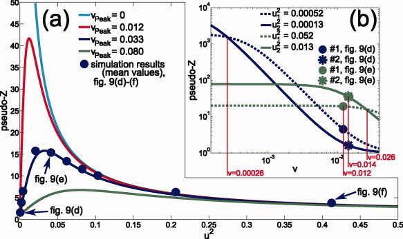
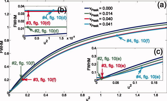
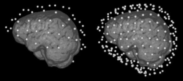
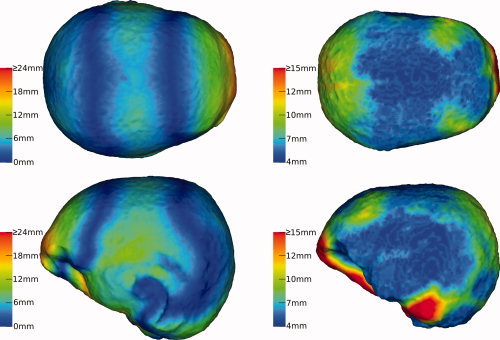
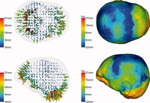
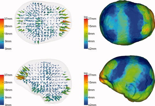
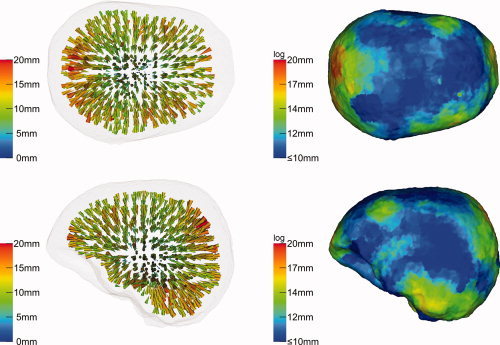
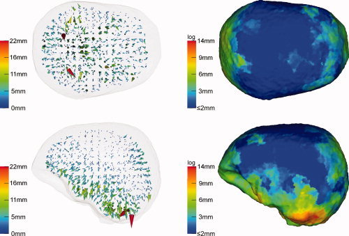
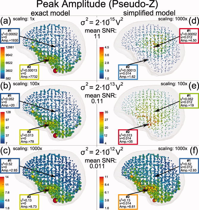
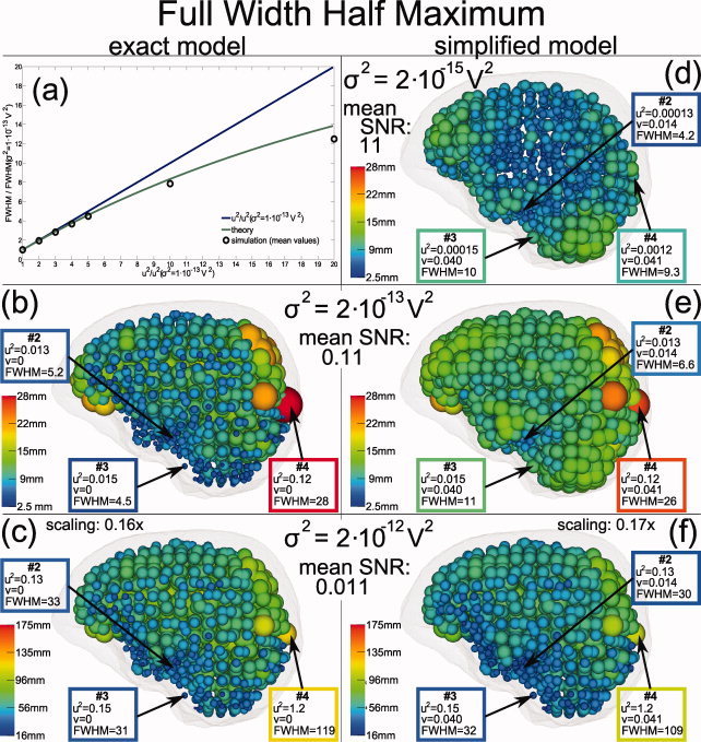
Beamforming approaches have recently been developed for the field of electroencephalography (EEG) and magnetoencephalography (MEG) source analysis and opened up new applications within various fields of neuroscience. While the number of beamformer applications thus increases fast-paced, fundamental methodological considerations, especially the dependence of beamformer performance on leadfield accuracy, is still quite unclear. In this article, we present a systematic study on the influence of improper volume conductor modeling on the source reconstruction performance of an EEG-data based synthetic aperture magnetometry (SAM) beamforming approach. A finite element model of a human head is derived from multimodal MR images and serves as a realistic volume conductor model. By means of a theoretical analysis followed by a series of computer simulations insight is gained into beamformer performance with respect to reconstruction errors in peak location, peak amplitude, and peak width resulting from geometry and anisotropy volume conductor misspecifications, sensor noise, and insufficient sensor coverage. We conclude that depending on source position, sensor coverage, and accuracy of the volume conductor model, localization errors up to several centimeters must be expected. As we could show that the beamformer tries to find the best fitting leadfield (least squares) with respect to its scanning space, this result can be generalized to other localization methods. More specific, amplitude, and width of the beamformer peaks significantly depend on the interaction between noise and accuracy of the volume conductor model. The beamformer can strongly profit from a high signal-to-noise ratio, but this requires a sufficiently realistic volume conductor model.

Figure 1

Theoretical pseudo‐Z curves: (a) u ² ↦ Z ² for local modeling errors v _peak found for the simulations presented in Figures 9 and 10 [exact model (v _peak = 0) and simplified model at minimum (0.012), mean (0.033), and maximum (0.080) of v _peak]. The blue disks show simulation results (means across all sources, cf. Fig. 9) for different noise levels (including the noise levels presented in Fig. 9): σ² = 2, 10, 20, 100, 200, 300, 400, 500, 1000, 2000 × 10⁻¹⁵ V². (b) v ↦ Z ² (logarithmic scales) for the sources #1 (disk) and #2 (asterisk) of the simulations highlighted in Figure 9d, blue curves, and Figure 9e, green curves. [Color figure can be viewed in the online issue, which is available at wileyonlinelibrary.com.]

Figure 2

Theoretical FWHM curves in dependence of the noise parameter u ² for four different local modeling errors v _peak found for the simulations presented in Figure 10: v _peak = 0 (blue curve) for the exact model; v _peak = 0.014 (green curve), v _peak = 0.040 (red curve), and v _peak = 0.041 (cyan curve) for the example sources #2, #3, and #4 reconstructed by using the simplified model (cf. Fig. 10). (b) and (c) show magnifications of the curves in (a): The ranges of u ² values shown in (a), (b), and (c) result from the simulations shown in Figure 10f, e, and d, respectively. [Color figure can be viewed in the online issue, which is available at wileyonlinelibrary.com.]

Figure 3

The two sensor configurations used in this study: A realistic sensor cap with 71 electrodes based on the international 10‐10 system and a synthetic sensor configuration with 258 sensors covering the complete head.

Figure 4

Geometrical properties of the FE models: The left column illustrates the local deviation between the FE outer skin surface and its approximation by the spherical head model. The right column visualizes the local thickness of the skull. [Color figure can be viewed in the online issue, which is available at wileyonlinelibrary.com.]

Figure 5

Beamformer (SAM) reconstruction inaccuracies as mere consequence of geometrical modeling imprecision if based on realistic sensor coverage (10‐10 system): An isotropically conducting FE model has been used for the forward solution while the inverse reconstruction was based on an isotropically conducting spherical head model. The left column illustrates the reconstruction results for each simulated dipole as three‐dimensional field of displacement vectors (cones). The right column visualizes the superficial reconstruction errors as projection to the outer skin surface. [Color figure can be viewed in the online issue, which is available at wileyonlinelibrary.com.]

Figure 6

Beamformer (SAM) reconstruction inaccuracies due to geometrical errors if based on a synthetic full coverage sensor configuration—otherwise identical to simulation shown in Figure 5. [Color figure can be viewed in the online issue, which is available at wileyonlinelibrary.com.]

Figure 7

Beamformer (SAM) reconstruction inaccuracies due to skull anisotropy: Volume constraint. Forward model: 1:10 anisotropic FEM with volume constraint (skull conductivity: μ_rad = 0.000905 S/m, μ_tang = 0.00905 S/m). Inverse model: Isotropic FEM (skull conductivity of 0.0042 S/m). Sensor configuration: Full coverage (258 sensors). [Color figure can be viewed in the online issue, which is available at wileyonlinelibrary.com.]

Figure 8

Beamformer (SAM) reconstruction inaccuracies due to skull anisotropy: Increased tangential conductivity. Forward model: 1:10 anisotropic FEM (μ_rad = 0.0042 S/m, μ_tang = 0.042 S/m). Inverse model: isotropic FEM (skull conductivity of 0.0042 S/m). Sensor configuration: realistic 10‐10 sensor system. [Color figure can be viewed in the online issue, which is available at wileyonlinelibrary.com.]

Figure 9

Distribution of beamformer (SAM) peak amplitudes in dependence of noise level and modeling errors. Peak amplitudes are illustrated by sphere radii—note the different scalings. Sources were simulated within the FE model with 1:10 skull anisotropy (volume constraint). The left side illustrated SAM reconstruction results if the inverse modeling was based on this exact volume conductor model. On the right side, the beamformer reconstruction was based on a simplified volume conductor model: the associated isotropic FE model. From the top to the bottom row increasing noise levels were selected. Results for two sample sources, labeled #1 and #2, are emphasized, for which connected theoretical curves are presented in Figure 1. All calculations were based on the full coverage sensor configuration. [Color figure can be viewed in the online issue, which is available at wileyonlinelibrary.com.]

Figure 10

Distribution of the beamformer (SAM) peak widths for the same simulations as in Figure 9. Sphere radii correspond to FWHM peak widths—please note different scaling in bottom row. Results for three sample sources, labeled #2 (cf. Fig. 9), #3, and #4, are emphasized. Figure 2 compares these values with the theory. In Figure 10a mean FWHM values simulated with the exact model for different noise levels (black circles) are compared to the theoretical function (green curve). To allow a comparison of distance based simulation results and the leadfield deviation based theory, relative FWHM values (dimensionless) based on the noise level σ² = 1 × 10⁻¹³ V² are shown (see text). The blue curve illustrates a linear approximation of the theoretical function. [Color figure can be viewed in the online issue, which is available at wileyonlinelibrary.com.]

References

1. Baillet S, Mosher JC, Leahy RM ( 2001): Electromagnetic brain mapping. IEEE Signal Process Mag 18: 14–30.
1. Barnes GR, Hillebrand A ( 2003): Statistical flattening of MEG beamformer images. Hum Brain Mapp 18: 1–12. - PMC - PubMed
1. Barnes GR, Hillebrand A, Fawcett IP, Singh KD ( 2004): Realistic spatial sampling for MEG beamformer images. Hum Brain Mapp 23: 120–127. - PMC - PubMed
1. Bertrand O, Thévenet M, Perrin F ( 1991): 3D finite element method in brain electrical activity studies In: Nenoner J, Rajala HM, Katila T, editors. Biomagnetic Localization and 3D Modelling. Helsinki University of Technology, Helsinki, pp 154–171.
1. Brookes MJ, Gibson AM, Hall SD, Furlong PL, Barnes GR, Hillebrand A, Singh KD, Holliday IE, Francis ST, Morris PG ( 2004): A general linear model for MEG beamformer imaging. Neuroimage 23: 936–946. - PubMed
Publication types