A Spatio-Temporal Downscaler for Output From Numerical Models

Abstract

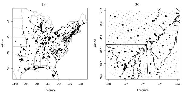
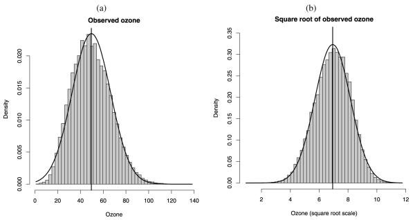
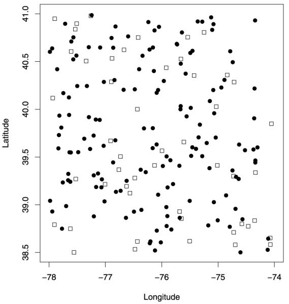
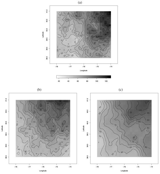
Often, in environmental data collection, data arise from two sources: numerical models and monitoring networks. The first source provides predictions at the level of grid cells, while the second source gives measurements at points. The first is characterized by full spatial coverage of the region of interest, high temporal resolution, no missing data but consequential calibration concerns. The second tends to be sparsely collected in space with coarser temporal resolution, often with missing data but, where recorded, provides, essentially, the true value. Accommodating the spatial misalignment between the two types of data is of fundamental importance for both improved predictions of exposure as well as for evaluation and calibration of the numerical model. In this article we propose a simple, fully model-based strategy to downscale the output from numerical models to point level. The static spatial model, specified within a Bayesian framework, regresses the observed data on the numerical model output using spatially-varying coefficients which are specified through a correlated spatial Gaussian process.As an example, we apply our method to ozone concentration data for the eastern U.S. and compare it to Bayesian melding (Fuentes and Raftery 2005) and ordinary kriging (Cressie 1993; Chilès and Delfiner 1999). Our results show that our method outperforms Bayesian melding in terms of computing speed and it is superior to both Bayesian melding and ordinary kriging in terms of predictive performance; predictions obtained with our method are better calibrated and predictive intervals have empirical coverage closer to the nominal values. Moreover, our model can be easily extended to accommodate for the temporal dimension. In this regard, we consider several spatio-temporal versions of the static model. We compare them using out-of-sample predictions of ozone concentration for the eastern U.S. for the period May 1-October 15, 2001. For the best choice, we present a summary of the analysis. Supplemental material, including color versions of Figures 4, 5, 6, 7, and 8, and MCMC diagnostic plots, are available online.

Figure 1

(a) Ozone monitoring sites in the Eastern U.S.; (b) Subset region used to compare ordinary kriging, Bayesian melding and the downscaler. The black points represent monitoring sites, the black dots represent the centroids of the CMAQ grid cells.

Figure 2

(a) Histogram of ozone observed at monitoring sites in the Eastern U.S. during the period May 1, 2001–October 15, 2001. (b) Histogram of square root of ozone. In each plot, a normal curve with mean and standard deviation, respectively, equal to the mean and standard deviation of the observed values and of the square root of the observed values is overlaid on the histogram.

Figure 3

Validation (squares) and test sites (black dots) used to assess the predictive performance of Bayesian melding and the downscaler on the simulated data.

Figure 4

(a) Simulated observed process at CMAQ grid cells, obtained by adding a white noise process, sampled from a N(0, 0.02) distribution, to the simulated true process. Predictive surface at CMAQ grid cells as obtained using: (b) Bayesian melding and (c) our downscaler. The legend for panels (a)–(c) is provided below panel (a). Color versions of panels (a)–(c) are available in the online appendix with supplemental material.

Figure 5

(a) Posterior predictive mean and (b) standard deviation for the spatially-varying additive bias, β₀(s) of the CMAQ output for August 11, 2001. Color versions of panels (a)–(b) are available in the online appendix with supplemental material.

Figure 6

(a) Observed ozone on August 11, 2001. Predicted ozone surface for August 11, 2001 as provided by: (b) CMAQ; (c) ordinary kriging; (d) Bayesian melding; and (e) the downscaler method. The legend for panels (a)–(e) is provided beside panel (a). Color versions of panels (a)–(e) are available in the online appendix with supplemental material.

Figure 6

(a) Observed ozone on August 11, 2001. Predicted ozone surface for August 11, 2001 as provided by: (b) CMAQ; (c) ordinary kriging; (d) Bayesian melding; and (e) the downscaler method. The legend for panels (a)–(e) is provided beside panel (a). Color versions of panels (a)–(e) are available in the online appendix with supplemental material.

Figure 7

(a) Posterior predictive mean and (b) posterior predictive standard deviation of the 4th highest ozone concentration during the period May 1–October 15, 2001. Color versions of panels (a)–(b) are available in the online appendix with supplemental material.

Figure 8

Posterior predictive probability that the 4th highest ozone concentration during the period May 1–October 15, 2001 is above (a) 75 ppb and (b) above 80 ppb. The dots show the observed occurrence that the 4th highest ozone concentration is above 75 ppb and 80 ppb, respectively. Color versions of panels (a)–(b) are available in the online appendix with supplemental material.

References

-
- Banerjee S, Carlin BP, Gelfand AE. Hierarchical Modeling and Analysis for Spatial Data. Chapman & Hall/CRC; Boca Raton, FL: 2004.
- Carroll SS, Day G, Cressie N, Carroll TR. Spatial Modeling of Snow Water Equivalent Using Airborne and Ground-Based Snow Data. Environmetrics. 1995;6:127–139.
- Carter C, Kohn R. On Gibbs Sampling for State Space Models. Biometrika. 1994;81:541–553.
- Chilès J-P, Delfiner P. Geostatistics: Modeling Spatial Uncertainty. Wiley; New York: 1999.
- Cowles MK, Zimmerman DL. A Bayesian Space-Time Analysis of Acid Deposition Data Combined From Two Monitoring Networks. Journal of Geophysical Research. 2003;108(D24):9006. doi: 10.1029/2003JD004001.
Grants and funding
LinkOut - more resources
Full Text Sources