The Viking viewer for connectomics: scalable multi-user annotation and summarization of large volume data sets

Abstract

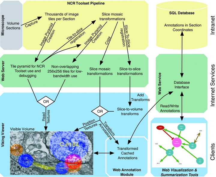
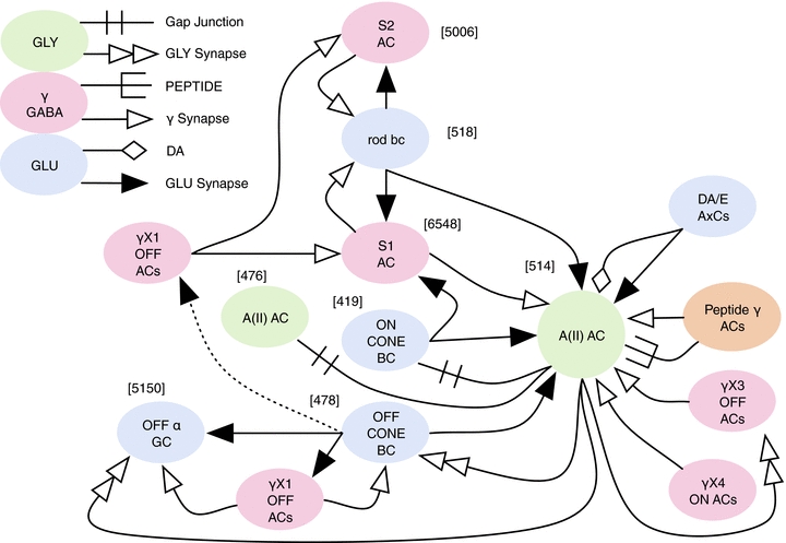
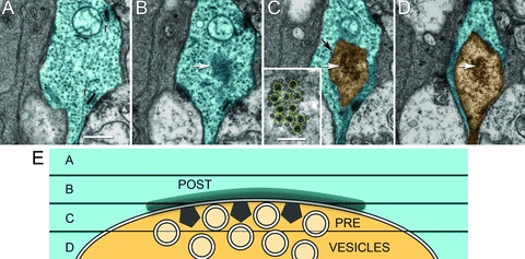
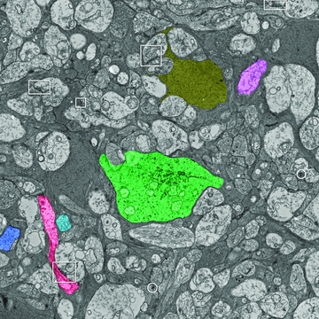
Modern microscope automation permits the collection of vast amounts of continuous anatomical imagery in both two and three dimensions. These large data sets present significant challenges for data storage, access, viewing, annotation and analysis. The cost and overhead of collecting and storing the data can be extremely high. Large data sets quickly exceed an individual's capability for timely analysis and present challenges in efficiently applying transforms, if needed. Finally annotated anatomical data sets can represent a significant investment of resources and should be easily accessible to the scientific community. The Viking application was our solution created to view and annotate a 16.5 TB ultrastructural retinal connectome volume and we demonstrate its utility in reconstructing neural networks for a distinctive retinal amacrine cell class. Viking has several key features. (1) It works over the internet using HTTP and supports many concurrent users limited only by hardware. (2) It supports a multi-user, collaborative annotation strategy. (3) It cleanly demarcates viewing and analysis from data collection and hosting. (4) It is capable of applying transformations in real-time. (5) It has an easily extensible user interface, allowing addition of specialized modules without rewriting the viewer.

Fig. 1

Overview of NCR Toolset and Viking systems. Viking provides a scalable environment for concurrent annotation, based on a three-tier architecture. Top-tier processing of the original data and database maintenance are performed on-site and need not be placed on the internet. Images, transforms, and a web services definition language (WSDL) interface form the middle tier to which a variety of client applications can be targeted. Client software includes our viewing/annotation client and visualization web site. Method calls between layers are stateless. Tiered designs allow modification of a layer without changes to the others, so long as the interfaces unchanged. Modular elements can be re-engineered if a new component is needed.

Fig. 2

Transform addition. To create a volume for three slices, we begin with two stos transforms mapping slice 2 to slice 1 (2 → 1) (A,B) and slice 3 to slice 2 (3 → 2) (C,D). Initial transforms are constructed by placing an even grid of mapped points on the slice to be transformed (B,D). Control points are located on the control slice by the NCR Toolset (A,C). Viking loads the transforms and creates a slice-to-volume transform by mapping control points on slice 2 from the 3 → 2 transform onto the 2 → 1 transform (E). In some cases, control points cannot not be mapped because they fall outside the defined grid transform. When this occurs, each line connecting the point to its neighbours, determined by Delaunay triangulation, is tested to see if it intersects with the edge of the grid transform (F). The mapped coordinates are moved along the corresponding line by the same relative distance (H). The mapped control points create a new set of control points which define the 3 → 1 transform (G), which would be the slice-to-volume transform for slice 3 (G,H). After a small number of slices are transformed into a volume the mapped coordinates converge to a circular shape.

Fig. 3

The Viking interface modes. (A) The Slice mode, selected at left tab window, allows selection of the slice to view in the right data window. Panning, zooming, and navigating forward or back a slice are mouse actions. Navigation is aided by keystroke shortcuts. This is a low-resolution (124 nm per pixel) view of an array of annotated cells (blue and green circles) in the inner nuclear layer of rabbit retinal connectome volume RC1. Individual structures (e.g. cells) all have Property Sheets for metadata logging and user guidance. (B) The Structure Type mode enables the annotation process. This is a high-resolution (6.6 nm per pixel) view of annotated processes and synapses. Figure 5 describes the annotation process. Property Sheets also have dynamically updated Location panels to guide navigation along a structure in X pixel, Y pixel Z slice space.

Fig. 5

Tracking workflow in Viking. (A,B) Viking screen captures show unmarked EM images of two adjacent serial slices numbered 152 (A) and 153 (B). A long amacrine cell (AC) process passes horizontally along the bottom of both images. It is broken into two isolated segments on slice 153. (C) Annotation of slice 152 shows the AC process as structure C5303 (small blue circle) with two associated postsynaptic densities where input is received from unlabeled conventional synapses. Triangles indicate the locations of annotations on adjacent slices. Yellow lines indicate links between locations. (D–F) Progressive annotations of slice 153. (D) The left-hand segment of amacrine cell is annotated C5303, but the right-hand segment is not. (E) The user extends the tracking of C5303 by dragging a line from the existing location on the adjacent slice (triangle) which creates a new location (right-hand blue circle), a link line (yellow) and an entry in the LocationLinks table linking them. The user then creates a structure for the post-synaptic density (orange circle) and associates it with C5303 (fine white link line). (F) At a later time, a user tracks cell C6184 and finds that it forms the presynaptic part of the synapse annotated in (E). A conventional synapse structure (red circle) is created for the presynaptic side and linked to both C6184 and the paired postsynaptic structure with a drag–drop operation.

Fig. 4

Multi-resolution and multi-channel support. (A,B) Low-magnification views of slice 61 (A) which contains a GABA overlay (red) captured with a 100× oil objective overlayed on the adjacent TEM section (cyan) and slice 152 (B) which contains a Glycine (green) overlayed on TEM (magenta). Note cell bodies containing GABA/Glycine are easily identified. (C,D) High-resolution views of from slice 182 w/GABA (C) and slice 152 with a Glycine overlay (D). Many fine processes can be identified as containing glycine or GABA. Brighter light microscopy overlays indicate higher concentrations of the target small molecule.

Fig. 6

The Viking annotation database SQL schema. Each box contains the table name (top panel), a list of columns (right panel), and whether the column serves as a key in the database (left panel). The functions of these tables are described in the Annotation Database portion of the methods. Primary keys are noted with PK, Foreign keys are denoted with FK. Column names listed in bold are required fields. Relations (lines) between tables are shown using Crow's foot notation.

Fig. 7

Rendering of cells in VikingPlot. Selected neurons connected in an A_II amacrine cell network were rendered with the VikingPlot, demonstrating their approximate morphologies in vertical (A) and horizontal (B) orientations. The A_II amacrine cells are numbered 476, 514, 2610 and 3679 in Fig. 8, which shows the connectivity graph. Cell classes are colour coded. A_II amacrine cells are shades of yellow. ON Bipolar cells are shades of green. OFF BCs are shades of blue. Rod bipolar cells are shades of purple. Unidentified processes are white. A long OFF α ganglion cell dendrite (C5150) entering from the right in (A) is coded red-orange. A process containing peptide vesicles (C6406) also enters from the right (A) slightly below and is colour light orange.

Fig. 8

Automatic generation of network graphs. The visualization web query (see ‘Materials and methods’) for cells connected to A_II amacrine cell 476 by three or fewer hops produces a directed graph with an automated ‘pretty’ layout for human interpretation. Nodes are colour coded according to cell type or are grey if type has not been assigned. Solitary numbers indicate that the graph continues past the requested hop limit. Edges are directed: green arrows represent ribbon synapses, red T-bars represent conventional synapses, yellow double headed arrows represent gap junctions. Labels: BC, bipolar cell; GC, ganglion cell; AC, amacrine cell; GBC, glycine immunopositive bipolar cell; PROCESS, element not yet classified.

Fig. 9

Network summary. Using automated network graphs, connectivity data were further condensed to present the connectivity of multiple A_II amacrine cells as a single human-interpretable summary. Combining CMP, morphological and ATEM connectivity observations makes it possible to classify cells in the observed network by multiple techniques in the same data set.

Fig. 10

Serial slices demonstrating the challenges in automated tracking. Oblique orientation synapses are common. Four adjacent 70 nm slices in the RC1 volume illustrate the problem, which cannot be solved by making slices thinner. (A) In slice 232, a bipolar cell process (cyan) is centred in the frame, with two ribbon (r) synapses. There are actually four oblique synapses in this series. We track only one. Scale for (A–D), 500 nm. (B) On slice 231, a central dark patch represents the bipolar cell's postsynaptic density (white arrow) to an amacrine cell input. (C) In slice 230, the amacrine cell process (orange) emerges in the centre of the contact zone (white arrow) along with its array of presynaptic projection densities (inset box, yellow circles, scale, 250 nm). The membranes between the amacrine cell and bipolar cell pass through the slice obliquely and appear as a dark circular smudges (black arrow). Presynaptic vesicles appear in the centre of the patch. (D) Slice 229 contains the amacrine cell process (orange) with its cluster of presynaptic vesicles (white arrow) rimmed by the bipolar cell (cyan). (E) An orthogonal view of the four-slice partitioning of a conventional synapse with the bipolar cell (cyan) postsynaptic density (POST) in slice B, the amacrine cell (orange) presynaptic projections (PRE) in slice C, and vesicles (circles) in slice D.

Fig. 11

A keyframe image for the RC1 514_ipl tracking challenge. Six cells have been manually masked off and they are numbered in order of difficulty, with cell #1 being the easiest to track. The goal is to track the labelled cells from any starting section to the edges of the challenge volume. The challenge volume was exported from Viking at full resolution and starts at slice 126 (location X 48888, Y 48888) in the inner plexiform layer of the retina, centred on A_II amacrine cell C514 (green). Selected processes are colour coded to guide initiation of tracking (yellow, Müller cell; blue, bipolar cell 1; cyan, bipolar cell 2; red, amacrine cell; purple, ganglion cell). A selection of some (not all) representative conventional (boxes) and ribbon (circles) synapses is also provided. The image is 17.8 μm wide.

References

1. Amari SI, Beltrame F, Bjaalie JG, et al. Neuroinformatics: the integration of shared databases and tools towards integrative neuroscience. J. Integr. Neurosci. 2002;1:117–128. - PubMed
1. Anderson JR, Jones BW, Yang J-H, et al. A computational framework for ultrastructural mapping of neural circuitry. PLoS Biol. 2009;7:e1000074. - PMC - PubMed
1. Fiala JC. Reconstruct: a free editor for serial section microscopy. J. Microsc. 2005;218:52–61. - PubMed
1. Gansner ER, North SC. An open graph visualization system and its applications to software engineering. Softw. – Pract. Exp. 1999;30:1203–1233.
1. Google. KML Reference – KML – Google Code. Google, Inc; 2010.
Publication types