Predictive markers for AD in a multi-modality framework: an analysis of MCI progression in the ADNI population

Abstract

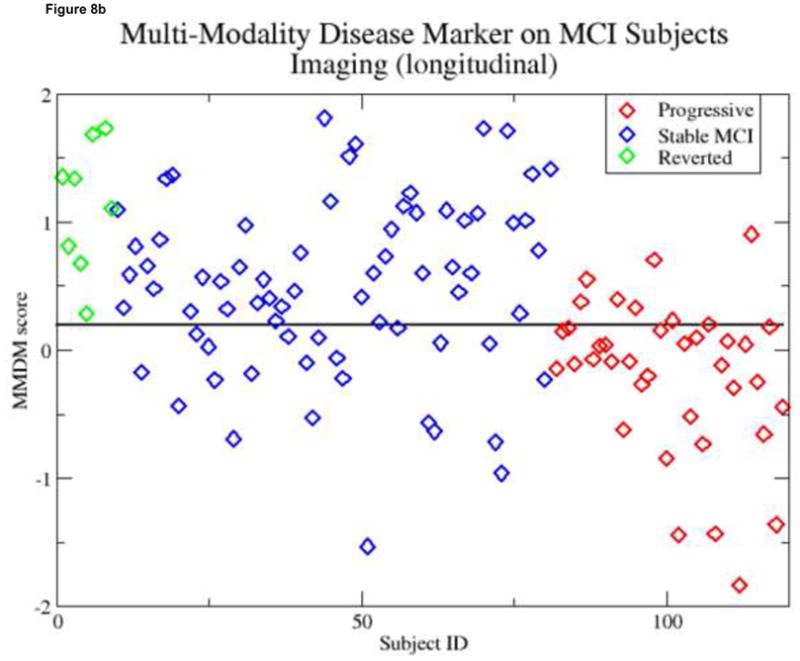
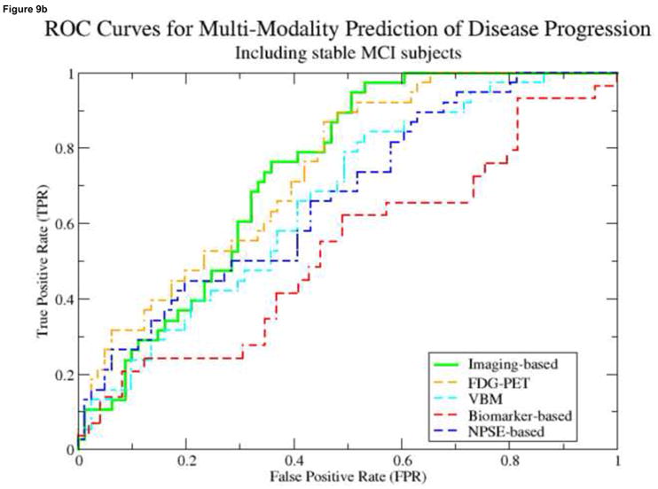
Alzheimer's Disease (AD) and other neurodegenerative diseases affect over 20 million people worldwide, and this number is projected to significantly increase in the coming decades. Proposed imaging-based markers have shown steadily improving levels of sensitivity/specificity in classifying individual subjects as AD or normal. Several of these efforts have utilized statistical machine learning techniques, using brain images as input, as means of deriving such AD-related markers. A common characteristic of this line of research is a focus on either (1) using a single imaging modality for classification, or (2) incorporating several modalities, but reporting separate results for each. One strategy to improve on the success of these methods is to leverage all available imaging modalities together in a single automated learning framework. The rationale is that some subjects may show signs of pathology in one modality but not in another-by combining all available images a clearer view of the progression of disease pathology will emerge. Our method is based on the Multi-Kernel Learning (MKL) framework, which allows the inclusion of an arbitrary number of views of the data in a maximum margin, kernel learning framework. The principal innovation behind MKL is that it learns an optimal combination of kernel (similarity) matrices while simultaneously training a classifier. In classification experiments MKL outperformed an SVM trained on all available features by 3%-4%. We are especially interested in whether such markers are capable of identifying early signs of the disease. To address this question, we have examined whether our multi-modal disease marker (MMDM) can predict conversion from Mild Cognitive Impairment (MCI) to AD. Our experiments reveal that this measure shows significant group differences between MCI subjects who progressed to AD, and those who remained stable for 3 years. These differences were most significant in MMDMs based on imaging data. We also discuss the relationship between our MMDM and an individual's conversion from MCI to AD.

Figure 1

Accuracies of single-kernel, single-modality methods. Color represents classification accuracy on unseen test data, ranging from blue (lowest, 50% accuracy,) to red (highest, 100% accuracy). The modalities used are, (a) FDG-PET scans at baseline, (b) VBM-processed MR baseline scans, (c) FDG-PET scans at 24 months, and (d) TBM-processed MR scans. See supplemental tables 8 – 11 for raw numbers.

Figure 1

Accuracies of single-kernel, single-modality methods. Color represents classification accuracy on unseen test data, ranging from blue (lowest, 50% accuracy,) to red (highest, 100% accuracy). The modalities used are, (a) FDG-PET scans at baseline, (b) VBM-processed MR baseline scans, (c) FDG-PET scans at 24 months, and (d) TBM-processed MR scans. See supplemental tables 8 – 11 for raw numbers.

Figure 1

Accuracies of single-kernel, single-modality methods. Color represents classification accuracy on unseen test data, ranging from blue (lowest, 50% accuracy,) to red (highest, 100% accuracy). The modalities used are, (a) FDG-PET scans at baseline, (b) VBM-processed MR baseline scans, (c) FDG-PET scans at 24 months, and (d) TBM-processed MR scans. See supplemental tables 8 – 11 for raw numbers.

Figure 1

Accuracies of single-kernel, single-modality methods. Color represents classification accuracy on unseen test data, ranging from blue (lowest, 50% accuracy,) to red (highest, 100% accuracy). The modalities used are, (a) FDG-PET scans at baseline, (b) VBM-processed MR baseline scans, (c) FDG-PET scans at 24 months, and (d) TBM-processed MR scans. See supplemental tables 8 – 11 for raw numbers.

Figure 2

Subkernel weights (β) chosen by the MKL algorithm with 2-norm regularization. Weights are relative, and have no applicable units. The modalities used are, (a) FDG-PET scans at baseline, (b) VBM-processed MR baseline scans, (c) FDG-PET scans at 24 months, and (d) TBM-processed MR scans.

Figure 2

Subkernel weights (β) chosen by the MKL algorithm with 2-norm regularization. Weights are relative, and have no applicable units. The modalities used are, (a) FDG-PET scans at baseline, (b) VBM-processed MR baseline scans, (c) FDG-PET scans at 24 months, and (d) TBM-processed MR scans.

Figure 2

Subkernel weights (β) chosen by the MKL algorithm with 2-norm regularization. Weights are relative, and have no applicable units. The modalities used are, (a) FDG-PET scans at baseline, (b) VBM-processed MR baseline scans, (c) FDG-PET scans at 24 months, and (d) TBM-processed MR scans.

Figure 2

Subkernel weights (β) chosen by the MKL algorithm with 2-norm regularization. Weights are relative, and have no applicable units. The modalities used are, (a) FDG-PET scans at baseline, (b) VBM-processed MR baseline scans, (c) FDG-PET scans at 24 months, and (d) TBM-processed MR scans.

Figure 3

Voxels used in the classifier for FDG-PET baseline images. Weights are relative, and have no applicable units. Blue indicates negative weights, associated with AD, while green indicates zero or neutral weight, while red indicates positively weighted regions associated with healthy status. Green bars in the axial and sagittal views correspond to coronal slices.

Figure 3

Voxels used in the classifier for FDG-PET baseline images. Weights are relative, and have no applicable units. Blue indicates negative weights, associated with AD, while green indicates zero or neutral weight, while red indicates positively weighted regions associated with healthy status. Green bars in the axial and sagittal views correspond to coronal slices.

Figure 3

Voxels used in the classifier for FDG-PET baseline images. Weights are relative, and have no applicable units. Blue indicates negative weights, associated with AD, while green indicates zero or neutral weight, while red indicates positively weighted regions associated with healthy status. Green bars in the axial and sagittal views correspond to coronal slices.

Figure 4

Voxels used in the classifier for FDG-PET images at 24 months. Weights are relative, and have no applicable units. Blue indicates negative weights, associated with AD, while green indicates zero or neutral weight, while red indicates positively weighted regions associated with healthy status. Green bars in the axial and sagittal views correspond to coronal slices.

Figure 4

Voxels used in the classifier for FDG-PET images at 24 months. Weights are relative, and have no applicable units. Blue indicates negative weights, associated with AD, while green indicates zero or neutral weight, while red indicates positively weighted regions associated with healthy status. Green bars in the axial and sagittal views correspond to coronal slices.

Figure 4

Voxels used in the classifier for FDG-PET images at 24 months. Weights are relative, and have no applicable units. Blue indicates negative weights, associated with AD, while green indicates zero or neutral weight, while red indicates positively weighted regions associated with healthy status. Green bars in the axial and sagittal views correspond to coronal slices.

Figure 5

Voxels used in the classifier for TBM-processed MR images. Weights are relative, and have no applicable units. Blue indicates negative weights, associated with AD, while green indicates zero or neutral weight, while red indicates positively weighted regions associated with healthy status. Green bars in the axial and sagittal views correspond to coronal slices.

Figure 5

Voxels used in the classifier for TBM-processed MR images. Weights are relative, and have no applicable units. Blue indicates negative weights, associated with AD, while green indicates zero or neutral weight, while red indicates positively weighted regions associated with healthy status. Green bars in the axial and sagittal views correspond to coronal slices.

Figure 5

Voxels used in the classifier for TBM-processed MR images. Weights are relative, and have no applicable units. Blue indicates negative weights, associated with AD, while green indicates zero or neutral weight, while red indicates positively weighted regions associated with healthy status. Green bars in the axial and sagittal views correspond to coronal slices.

Figure 6

Voxels used in the classifier for VBM-processed (GM density) MR images. Weights are relative, and have no applicable units. Blue indicates negative weights, associated with AD, while green indicates zero or neutral weight, while red indicates positively weighted regions associated with healthy status. Green bars in the axial and sagittal views correspond to coronal slices.

Figure 6

Voxels used in the classifier for VBM-processed (GM density) MR images. Weights are relative, and have no applicable units. Blue indicates negative weights, associated with AD, while green indicates zero or neutral weight, while red indicates positively weighted regions associated with healthy status. Green bars in the axial and sagittal views correspond to coronal slices.

Figure 6

Voxels used in the classifier for VBM-processed (GM density) MR images. Weights are relative, and have no applicable units. Blue indicates negative weights, associated with AD, while green indicates zero or neutral weight, while red indicates positively weighted regions associated with healthy status. Green bars in the axial and sagittal views correspond to coronal slices.

Figure 7

Voxel weights assigned by the MKL classifier when the outlier subjects were removed. (a) FDG-PET baseline images; (b) FDG-PET images at 24 months; (c) VBM-processed baseline MR images; (d) TBM-processed longitudinal MR scans.

Figure 7

Voxel weights assigned by the MKL classifier when the outlier subjects were removed. (a) FDG-PET baseline images; (b) FDG-PET images at 24 months; (c) VBM-processed baseline MR images; (d) TBM-processed longitudinal MR scans.

Figure 7

Voxel weights assigned by the MKL classifier when the outlier subjects were removed. (a) FDG-PET baseline images; (b) FDG-PET images at 24 months; (c) VBM-processed baseline MR images; (d) TBM-processed longitudinal MR scans.

Figure 7

Voxel weights assigned by the MKL classifier when the outlier subjects were removed. (a) FDG-PET baseline images; (b) FDG-PET images at 24 months; (c) VBM-processed baseline MR images; (d) TBM-processed longitudinal MR scans.

Figure 8

MMDMs applied to the MCI population. Subjects which remained stable are shown in blue; subjects which progressed to AD are shown in red; subjects which reverted to normal cognitive status are shown in green. In each figure, a line giving maximal post-hoc accuracy is shown. Note that in some cases, the best accuracy can be achieved by simply labeling all subjects as the majority class. In some cases, MMDM scores were truncated to ±2 so as to preserve the relative scales. On the left (a,c) are shown MMDMs based on information available at baseline. Note the homogeneity of the groups, leading to poor separability. Imaging-based MMDMs are shown a the top (a), while MMDMs based on NPSEs are shown below (c). On the right (b,d) are shown MMDMs based on all modalities available at 24 months. Note the improved separability between the progressing (red) and stable (blue) MCI subjects. Note that the imaging-based marker above (b) shows slightly greater separation of the 2 groups.

Figure 8

MMDMs applied to the MCI population. Subjects which remained stable are shown in blue; subjects which progressed to AD are shown in red; subjects which reverted to normal cognitive status are shown in green. In each figure, a line giving maximal post-hoc accuracy is shown. Note that in some cases, the best accuracy can be achieved by simply labeling all subjects as the majority class. In some cases, MMDM scores were truncated to ±2 so as to preserve the relative scales. On the left (a,c) are shown MMDMs based on information available at baseline. Note the homogeneity of the groups, leading to poor separability. Imaging-based MMDMs are shown a the top (a), while MMDMs based on NPSEs are shown below (c). On the right (b,d) are shown MMDMs based on all modalities available at 24 months. Note the improved separability between the progressing (red) and stable (blue) MCI subjects. Note that the imaging-based marker above (b) shows slightly greater separation of the 2 groups.

Figure 8

MMDMs applied to the MCI population. Subjects which remained stable are shown in blue; subjects which progressed to AD are shown in red; subjects which reverted to normal cognitive status are shown in green. In each figure, a line giving maximal post-hoc accuracy is shown. Note that in some cases, the best accuracy can be achieved by simply labeling all subjects as the majority class. In some cases, MMDM scores were truncated to ±2 so as to preserve the relative scales. On the left (a,c) are shown MMDMs based on information available at baseline. Note the homogeneity of the groups, leading to poor separability. Imaging-based MMDMs are shown a the top (a), while MMDMs based on NPSEs are shown below (c). On the right (b,d) are shown MMDMs based on all modalities available at 24 months. Note the improved separability between the progressing (red) and stable (blue) MCI subjects. Note that the imaging-based marker above (b) shows slightly greater separation of the 2 groups.

Figure 8

MMDMs applied to the MCI population. Subjects which remained stable are shown in blue; subjects which progressed to AD are shown in red; subjects which reverted to normal cognitive status are shown in green. In each figure, a line giving maximal post-hoc accuracy is shown. Note that in some cases, the best accuracy can be achieved by simply labeling all subjects as the majority class. In some cases, MMDM scores were truncated to ±2 so as to preserve the relative scales. On the left (a,c) are shown MMDMs based on information available at baseline. Note the homogeneity of the groups, leading to poor separability. Imaging-based MMDMs are shown a the top (a), while MMDMs based on NPSEs are shown below (c). On the right (b,d) are shown MMDMs based on all modalities available at 24 months. Note the improved separability between the progressing (red) and stable (blue) MCI subjects. Note that the imaging-based marker above (b) shows slightly greater separation of the 2 groups.

Figure 9

ROC curves for multi-modality learning on disease progression of MCI subjects using various disease markers. The ROC curves for separating progressing and reverting MCI subjects on the left (a,c). The ROC curves for separating progressing MCI subjects from all others are shown on the right, (b,d). The top row (a,b) shows the curves derived from information available at baseline, while those on the bottom (c,d) were derived from scans and markers taken at both baseline and 24-months.

Figure 9

ROC curves for multi-modality learning on disease progression of MCI subjects using various disease markers. The ROC curves for separating progressing and reverting MCI subjects on the left (a,c). The ROC curves for separating progressing MCI subjects from all others are shown on the right, (b,d). The top row (a,b) shows the curves derived from information available at baseline, while those on the bottom (c,d) were derived from scans and markers taken at both baseline and 24-months.

Figure 9

ROC curves for multi-modality learning on disease progression of MCI subjects using various disease markers. The ROC curves for separating progressing and reverting MCI subjects on the left (a,c). The ROC curves for separating progressing MCI subjects from all others are shown on the right, (b,d). The top row (a,b) shows the curves derived from information available at baseline, while those on the bottom (c,d) were derived from scans and markers taken at both baseline and 24-months.

Figure 9

ROC curves for multi-modality learning on disease progression of MCI subjects using various disease markers. The ROC curves for separating progressing and reverting MCI subjects on the left (a,c). The ROC curves for separating progressing MCI subjects from all others are shown on the right, (b,d). The top row (a,b) shows the curves derived from information available at baseline, while those on the bottom (c,d) were derived from scans and markers taken at both baseline and 24-months.

References

1. Albert MS, Moss MB, Tanzi R, Jones K. Preclinical prediction of AD using neuropsychological tests. Journal of the International Neuropsychological Society. 2001;7(05):631–639. - PubMed
1. Arimura H, Yoshiura T, Kumazawa S, Tanaka K, Koga H, Mihara F, Honda H, Sakai S, Toyofuku F, Higashida Y. Automated method for identification of patients with Alzheimer’s disease based on three-dimensional MR images. Academic Radiology. 2008;15(3):274–284. - PubMed
1. Ashburner J. A fast diffeomorphic image registration algorithm. Neuroimage. 2007;38(1):95–113. - PubMed
1. Ashburner J, Friston KJ. Voxel-Based Morphometry - The Methods. Neuroimage. 2000;11(6):805–821. - PubMed
1. Bakir G, Hofmann T, Schölkopf B. Predicting structured data. The MIT Press; 2007.
Publication types