. 2010 Dec 8;30(49):16741-54.
doi: 10.1523/JNEUROSCI.2016-10.2010.

Cortical processing of dynamic sound envelope transitions

Affiliations

Cortical processing of dynamic sound envelope transitions

Yi Zhou et al. J Neurosci. .

Abstract

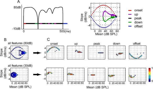
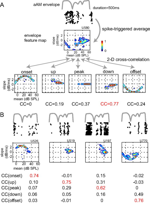
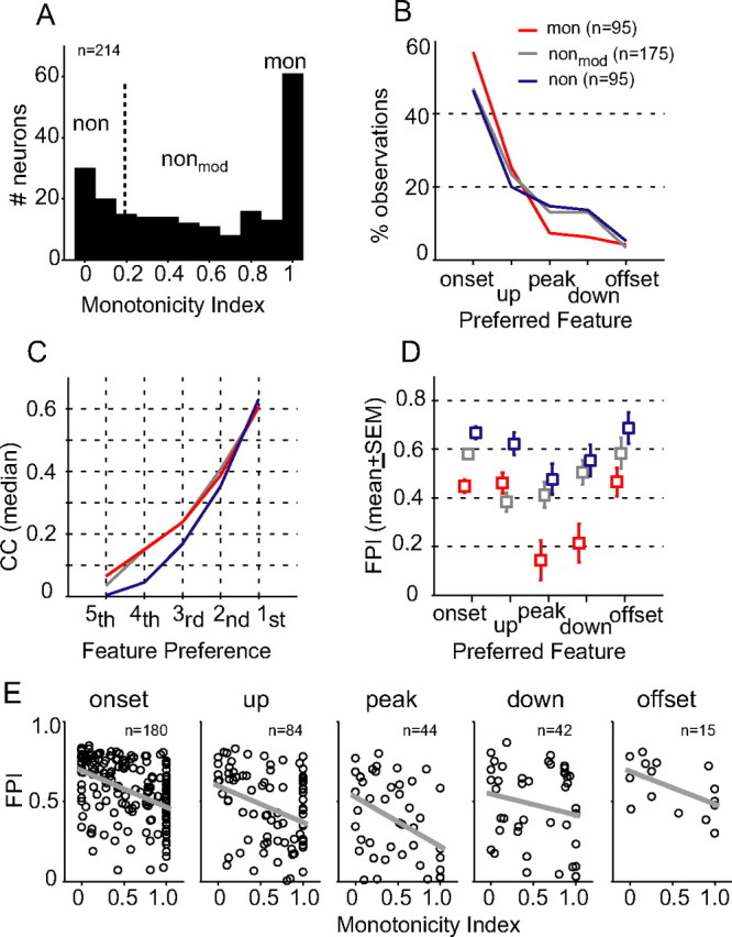
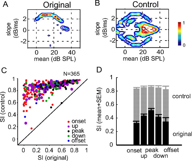
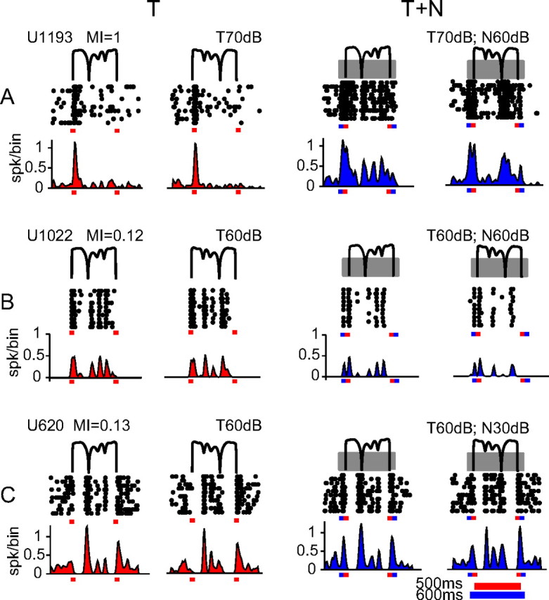
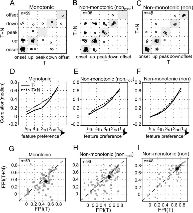
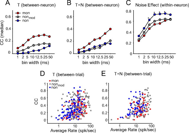
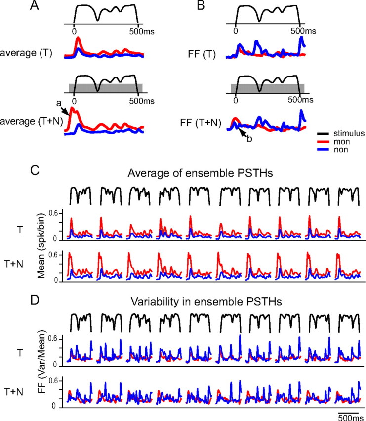
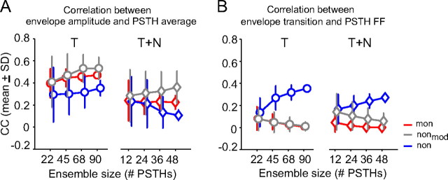
Slow envelope fluctuations in the range of 2-20 Hz provide important segmental cues for processing communication sounds. For a successful segmentation, a neural processor must capture envelope features associated with the rise and fall of signal energy, a process that is often challenged by the interference of background noise. This study investigated the neural representations of slowly varying envelopes in quiet and in background noise in the primary auditory cortex (A1) of awake marmoset monkeys. We characterized envelope features based on the local average and rate of change of sound level in envelope waveforms and identified envelope features to which neurons were selective by reverse correlation. Our results showed that envelope feature selectivity of A1 neurons was correlated with the degree of nonmonotonicity in their static rate-level functions. Nonmonotonic neurons exhibited greater feature selectivity than monotonic neurons in quiet and in background noise. The diverse envelope feature selectivity decreased spike-timing correlation among A1 neurons in response to the same envelope waveforms. As a result, the variability, but not the average, of the ensemble responses of A1 neurons represented more faithfully the dynamic transitions in low-frequency sound envelopes both in quiet and in background noise.


Figures

Figure 1.
Figure 1.
Envelope features of the aAM stimuli. A, Envelope of an aAM stimulus with a peak level of 80 dB SPL (left) and its mean–slope trajectory (right). Envelope segments with positive, zero, and negative slope values and their associated mean–slope trajectories are plotted in different colors. Each color dot on the mean–slope trajectory marks the mean–slope values of one 25 ms envelope segment. B, Contour plots of the mean–slope distributions of total envelope features in 10 aAM stimuli played at 80 and 30 dB SPL. C, Contour plots of the mean–slope distributions of five envelope feature types at 80 and 30 dB SPL. The color of a contour line indicates the peak-normalized magnitude of a distribution.
Figure 2.
Figure 2.
Characterization of envelope feature selectivity of A1 neurons. A, Shown from top to bottom are the envelope of an aAM stimulus at 60 dB SPL, the raster plot of corresponding responses of an example neuron, its envelope feature map, and the mean–slope distributions of five feature types of aAM stimuli at 60 dB SPL. The preferred feature type of a neuron was determined by the strength of the two-dimensional (2-D) correlation between the envelope feature map of a neuron and the mean–slope distributions of five envelope feature types. As highlighted in red, the down type yielded the highest CC and was then designated as the preferred envelope feature of this neuron. B, Raster plots and envelope feature maps of four other example neurons whose ID numbers are shown on top of feature maps. Based on the maximal strengths of correlation values with five envelope feature types (red), the preferred envelope feature types for the four example neurons from left to right are onset, up, peak, and offset. The peak SPLs used were 40 dB SPL for the onset and offset neurons, 60 dB SPL for the up neuron, and 50 dB SPL for the peak neuron. The FPI of the five neurons was in turn 0.63, 0.56, 0.66, 0.63, and 0.63. The aAM waveform lasted 500 ms and neural responses between 15 ms after the stimulus onset and 65 ms after the stimuli offset were analyzed. The raster plots were advanced 15 ms to visually align with the envelope of the aAM stimulus.
Figure 3.
Figure 3.
Comparison of envelope feature selectivity between monotonic and nonmonotonic neurons. A, Distribution of MI. For data analyses, the neural population was divided into three subgroups based on MI values (Table 1). B, Percentage of observations of feature types for the three neural groups. Neurons that were tested at more than one SPL contributed multiple observations. C, Ordered correlation coefficients (median) between stimulus-response feature maps, as demonstrated in Figure 2. The highest rank (first) is associated with the preferred feature type of a neuron. D, FPI (mean ± SEM) of monotonic (red), moderately nonmonotonic (gray), and highly nonmonotonic neurons (blue) for each feature type. E, Scatter plots of FPI as a function of MI for five feature types. Gray, Best-fit linear regression.
Figure 4.
Figure 4.
Envelope slope sensitivity of neurons in auditory cortex. A, B, Original (A) and control (B) feature maps of an example neuron. Highly asymmetric activity was observed in the original map, but not in the control obtained from shuffled spike times. C, Scatter plot of SI in the original (abscissa) and in the control map (ordinate) for all neurons tested. Different preferred envelope feature types are labeled in different colors. D, SI values (mean + SEM) of the original (black) and control (gray) feature maps for each feature type.
Figure 5.
Figure 5.
Spike-timing patterns to aAM envelope in background noise. A–C, Raster plots and PSTHs of responses of three neurons in T and T+N conditions. The envelopes of two aAM stimuli (forward and time-reversed) are shown in thin black lines above the raster plots. The ID number and MI value of a neuron and the SPLs of aAM and noise are indicated above the stimuli. To provide a visible reference for the noise responses, we intentionally chose these neurons showing excitatory responses to the noise onset. In the T+N condition, the broadband noise (depicted as gray blocks overlaying the aAM stimuli) was gated on 50 ms before the aAM onset and gated off 50 ms after the aAM offset. The onset and offset times are indicated by tick marks on each panel (aAM in red and noise in blue). Each aAM waveform lasted 500 ms and noise lasted 600 ms. The bin width used for PSTHs was 10 ms.
Figure 6.
Figure 6.
Comparison of envelope feature selectivity in background noise. A–C, Scatter plot of the preferred feature types of monotonic, moderately nonmonotonic, and highly nonmonotonic neurons tested in both T and T+N conditions. Each circle designates the preferred envelope types of one neuron with and without background noise in response to the same aAM stimuli. The median noise level was 40 dB SPL for all three neuronal populations. For the purpose of plotting, the five feature types were numbered from 1 to 5. For example, the onset–onset transition was positioned (1,1) on the x,y plane. To visually separate the circles within each subgrid, we jittered the position of each circle by adding a small Gaussian random number (mean = 0 and SD = 0.1) to its numerical feature type. D–F, Correlation coefficient (median) between stimulus–response feature maps in T and T+N conditions. Data are presented in the same format as those in Figure 3C. G–I, Scatter plot of FPI values between T and T+N conditions for individual neurons. The median FPI value is marked by a cross sign on each panel.
Figure 7.
Figure 7.
Correlation analysis of spike-timing patterns in response to aAM stimuli. A,B, The Pearson CC (median) of the between-neuron comparison in T and T+N conditions. C, The Pearson CC (median) of the within-neuron comparison between T and T+N conditions. *p < 0.05. In A–C, the spike times were binned at multiple resolutions ranging from 1 to 50 ms. Due to the temporal smoothing effect of a spike counting window, the correlation computed from PSTHs increased with the bin width. D,E, The Pearson CC of the between-trial comparison as a function of average rate in T and T+N conditions. Each circle represents data from one neuron, averaged over CCs from all pairwise correlations between different trials of responses. The PSTH bin width was 10 ms. The total numbers of PSTHs (i.e., test conditions) used in T and T+N conditions are listed in Table 1.
Figure 8.
Figure 8.
aAM envelope representation by a population of neurons. A,B, Average (A) and FF (B) of ensemble PSTHs for monotonic (red) and highly nonmonotonic neurons (blue) in response to an aAM envelope in T and T+N conditions. C,D, Average (C) and FF (D) of ensemble PSTHs to the 10 aAM envelopes in T and T+N conditions. The aAM duration was 500 ms and noise duration was 600 ms. The PSTHs show responses occurring from 100 ms before the aAM onset to 50 ms after the aAM offset (spike times were advanced 15 ms in data analyses). The PSTH bin width was 10 ms. The ensemble sizes in T and T+N conditions were the same as those in Figure 7.
Figure 9.
Figure 9.
Representation of envelope amplitude and transition by a population of neurons. A, Correlation coefficient (mean ± SD) between envelope amplitude and the average of ensemble PSTHs in T and T+N conditions. B, Correlation coefficient (mean ± SD) between envelope transition and the FF of ensemble PSTHs in T and T+N conditions. The envelope transitions were described by absolute values of the time derivative of aAM amplitude with a 1 ms time resolution. Individual PSTHs, envelope amplitude, and envelope transition were smoothed using a 10 ms time window before the correlation analysis. A bootstrap method was used to take repeated samples from the total PSTHs to form an ensemble. The ensemble size had approximately an incremental step of a quarter of the total PSTHs collected at each condition for monotonic and highly nonmonotonic neurons. The total numbers of PSTHs (i.e., test conditions) for each neuronal group were the same as those in Figures 7 and 8 and are listed in Table 1.

Similar articles

Cited by

References

    1. Bieser A, Müller-Preuss P. Auditory responsive cortex in the squirrel monkey: neural responses to amplitude-modulated sounds. Exp Brain Res. 1996;108:273–284. - PubMed
    1. Bregman AS. Auditory scene analysis: the perceptual organization of sound. Cambridge: MIT; 1990.
    1. Cariani P. As if time really mattered: temporal strategies for neural coding of sensory information. Commun Cogn Artif Intell. 1995;12:161–229.
    1. de Boer E, de Jongh HR. On cochlear encoding: potentialities and limitations of the reverse-correlation technique. J Acoust Soc Am. 1978;63:115–135. - PubMed
    1. deCharms RC, Merzenich MM. Primary cortical representation of sounds by the coordination of action-potential timing. Nature. 1996;381:610–613. - PubMed

Publication types