Self-organized criticality in developing neuronal networks

Abstract

Recently evidence has accumulated that many neural networks exhibit self-organized criticality. In this state, activity is similar across temporal scales and this is beneficial with respect to information flow. If subcritical, activity can die out, if supercritical epileptiform patterns may occur. Little is known about how developing networks will reach and stabilize criticality. Here we monitor the development between 13 and 95 days in vitro (DIV) of cortical cell cultures (n = 20) and find four different phases, related to their morphological maturation: An initial low-activity state (≈19 DIV) is followed by a supercritical (≈20 DIV) and then a subcritical one (≈36 DIV) until the network finally reaches stable criticality (≈58 DIV). Using network modeling and mathematical analysis we describe the dynamics of the emergent connectivity in such developing systems. Based on physiological observations, the synaptic development in the model is determined by the drive of the neurons to adjust their connectivity for reaching on average firing rate homeostasis. We predict a specific time course for the maturation of inhibition, with strong onset and delayed pruning, and that total synaptic connectivity should be strongly linked to the relative levels of excitation and inhibition. These results demonstrate that the interplay between activity and connectivity guides developing networks into criticality suggesting that this may be a generic and stable state of many networks in vivo and in vitro.

Figure 1. Raster plots at different temporal resolutions for experimental and model data.

They are showing (A) the patterns of high burst-like activity and following pauses and (B,C) the activity patterns during some bursts. For graphical reasons, in panels (B,C) intervals between bursts have been shortened and do not correspond to the true intervals visible in panel (A). Thus scale bars refer only to the bursts.

Figure 2. Development of the deviation from a power law of cell cultures.

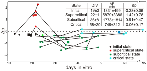
The transitions from initial (black) to supercritical (red) to subcritical (green) and critical state (blue) can be clearly seen. Data from the same cell culture at different time points are connected. 14% of the total number of cultures has been tracked at 5 different time points, 7% at 4 time points, 29% at 3, 14% at 2, and 36% once. Squares indicate the mean values of DIV and ( indicates the standard deviation), which are given in the inset Table, of the associated state. amount of action potentials per minute, therefore, mean activity.

Figure 3. Avalanche distribution changes during morphological development of dissociated cell cultures.

The dashed line indicates a perfect power law distribution. The deviation of the cell culture data from this line measures the criticality of these systems. For each state three different examples are shown. The age of each state of the cell cultures is given in the bottom right corner of the panels. (A) Initial state (on average 19 DIV); (B) supercritical state showing a “bump” of many long avalanches (on average 22 DIV); (C) subcritical state (on average 36 DIV) showing a depression and hence a lack of long avalanches; and (D) critical state (on average 58 DIV) with a good match to the power law line.

Figure 4. The development of the model shows three different phases (Phase I, II and III).

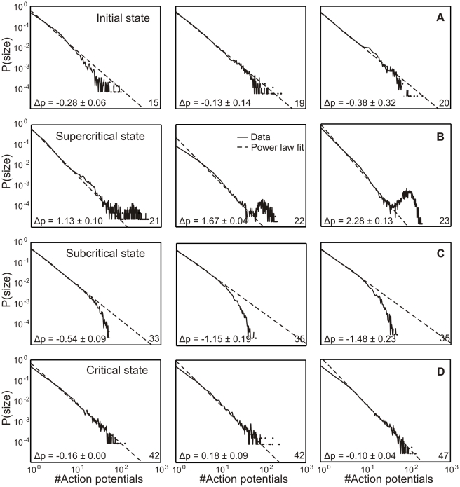
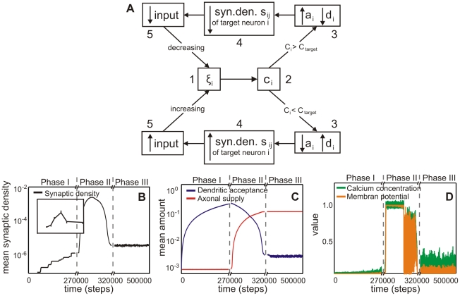
(A) Box diagram of the model feedback loop. Variables are membrane potential , calcium concentration , axonal supply and dendritic acceptance , and connectivity between dendrite and axon and the constant homeostatic value . The up and down arrows indicate if a variable is increased/decreased. For details see main text. (B) The mean synaptic density develops comparable to experimental findings in cell cultures (see inset from [24]). Note, time axis has been stretched in the middle. (C) Development of the average axonal supplies and dendritic acceptances. The network model passes through three different developmental phases: the first phase is characterized by a pronounced increase of the dendritic acceptance. During development, the network undergoes a transition (second phase) and finally it reaches a homeostatic equilibrium (third phase) with more axonal supplies than dendritic acceptances. (D) Network activity and calcium concentration change accordingly. At the beginning, activity rises slowly until a transition happens. During the transition, activity reaches its maximum and subsequently decreases to a homeostatic value.

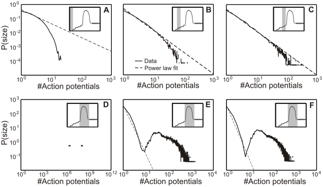
Figure 5. Avalanche distribution of the model in Phase I and II.

Gray areas in insets (taken from Figure 4 B) show the time point in the development. (top): (A) Initially, the connectivity between neurons is zero. Because of that a Poisson-like distribution describes the spontaneous neuronal activity best. (B,C) With increasing (B: ; C: ), the avalanche distribution turns from a Poisson into a power-law like distribution similar to Figure 3 A. (bottom): In Phase II without inhibition (D), no real avalanche distribution can be observed and one sees only one or two “avalanches” (marked by a cross). Adding inhibition brings the system back into a stable, albeit supercritical regime. Within a wide tested range (Table 2), the amount of inhibition does not significantly change the degree of supercriticality. (E) Network with weak inhibition and (F) with strong inhibition .

Figure 6. In the homeostatic equilibrium (Phase III), the degree of inhibition determines whether the network finally reaches a critical state or remains sub- or supercritical.

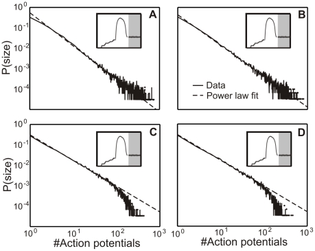
As a characteristic example the avalanche distributions from fixed point 1 (see Table 3) are shown. (A) A purely excitatory network stays slightly supercritical although network activities are homeostatically balanced (). (B) If the absolute value of the inhibitory strength equals the excitatory strength the network becomes critical (). Here the total number of inhibitory synapses is about 20%. (C–D) Higher levels of inhibition ( for C and for D) keep the network in a subcritical regime (C: ; D: ).

Figure 7. A sudden change of the inhibition in Phase III destabilizes the system.

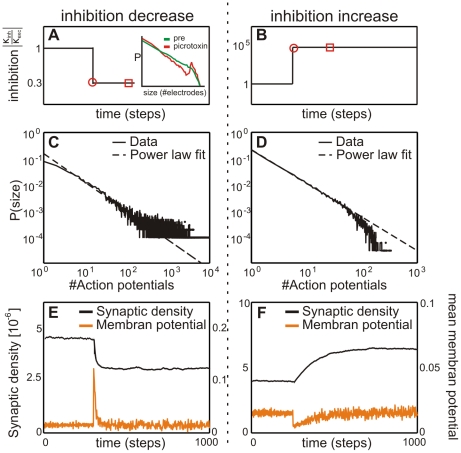
Inhibition is suddenly decreased/increased (left/right column) as shown in panels (A) and (B). After the jump, the avalanche distribution becomes (C) supercritical ( or (D) subcritical (), respectively. Distributions were plotted at the time point marked by the open disks in A and B. The reduced inhibition case is well backed-up by experimental data as a similar change in criticality was observed in mature cell cultures after artificially increasing inhibition (compare inset). After some time (open square marker) distributions change and are then those shown in panels A and D in Figure 6. Now we have in both cases somewhat reduced (absolute) values as compared to those directly after the jump (now for the supercritical case Figure 6 A and for the subcritical case Figure 6 D). Note, however, that we do not get back to the initial criticality (Figure 6 B, ). Parallel to this, the bottom panels (E,F) show that in both cases connectivity remains also changed. Activity, on the other hand, fully builds back.

Figure 8. Development of the network in phase space.

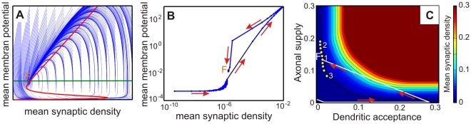
(A) Here the hysteresis curve of the mean membrane potential against the mean connectivity described by Equation 10 is displayed together with its possible trajectories (blue). marks the equilibrium or stable point of the network. (B) Hysteresis curve from the simulation. (C) Different representation, which shows that the equilibrium represents a region of fixed points with approximately equal connectivity. The axes represent here axonal supply and dendritic acceptance. Color indicates the calculated average connectivity . Depending on the initial state, the model grows into a fixed point of an omega limit set (yellow circles, region ) lying on a hyperbola (dashed line), thus with approximately equal connectivity . The “bumpy” shape of the hyperbola is due to grid aliasing effects.

Figure 9. Comparing real data (top) with model (bottom).

(A) Initial phase, (B) supercritical phase, (C) subcritical phase, and (D) critical phase.

Figure 10. Additional tests for criticality used for cell cultures and model.

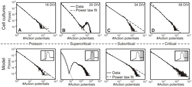
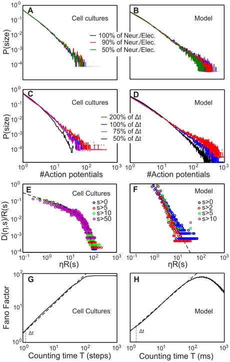
In (A,B) we address potential spatial non-stationarity effects by comparing distributions obtained with only certain percentage subsets of the electrodes (neurons). In (C,D) we show that only minor variations exist for different time bins. Thus, temporal non-stationarities on a short time scale appear unlikely. Panels (E,F) show the scaling function and, therefore, the scale-free behavior of model and cell cultures. Panels (G,H) show a Fano factor analysis for cell culture and model in the critical state. The exponent of the Fano Factor (linear regression) is for the model and for cell cultures. Hence we conclude a scale-free clustering over different time scales .

References

-
- Chialvo D. Critical brain networks. Physica A. 2004;340:756–765.
- Plenz D, Thiagarajan T. The organizing principles of neuronal avalanches: Cell assemblies in the cortex. Trends Neurosci. 2007;30:101–110. - PubMed
- Gutenberg B, Richter C. Seismicity of the earth. Princeton: Princeton University Press; 1956. 273
- Harris T. The theory of branching processes. New York: Dover Publications; 1989. 230
Publication types
MeSH terms
LinkOut - more resources
Full Text Sources