A Comparison between Mechanisms of Multi-Alternative Perceptual Decision Making: Ability to Explain Human Behavior, Predictions for Neurophysiology, and Relationship with Decision Theory

Abstract

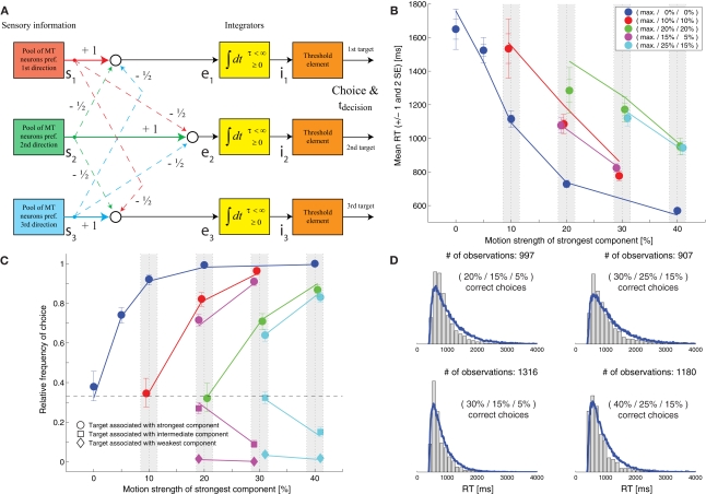
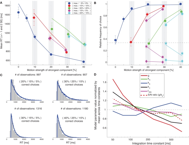
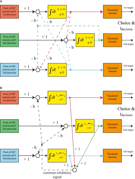
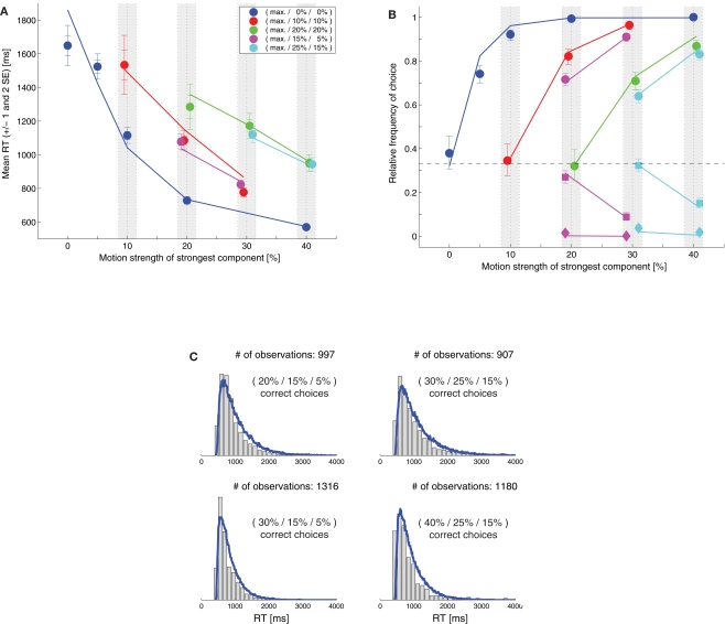
While there seems to be relatively wide agreement about perceptual decision making relying on integration-to-threshold mechanisms, proposed models differ in a variety of details. This study compares a range of mechanisms for multi-alternative perceptual decision making, including integration with and without leakage, feedforward and feedback inhibition for mediating the competition between integrators, as well as linear and non-linear mechanisms for combining signals across alternatives. It is shown that a number of mechanisms make very similar predictions for the decision behavior and are therefore able to explain previously published data from a multi-alternative perceptual decision task. However, it is also demonstrated that the mechanisms differ in their internal dynamics and therefore make different predictions for neuorphysiological experiments. The study further addresses the relationship of these mechanisms with decision theory and statistical testing and analyzes their optimality.

Keywords: behavior; decision theory; mathematical models; multiple alternatives; neurophysiology; perceptual decisions.

Figure 1

Slightly leaky feedforward inhibition model. (A) Structure of the model. Solid lines indicate excitatory connections, dashed lines inhibitory connections. (B) Fit of the model (lines) to the mean response time data (symbols). The coherence of the strongest motion component is plotted on the horizontal axis. The color codes for the strengths of the other two components. Data points within the light gray bars, which would normally all be aligned with the center of the bar, have been shifted horizontally for presentation purposes to reduce overlap. (C) Comparison between the model's choice predictions (lines) and the behavioral data (symbols). The error bars indicate 95% confidence intervals. (D) Comparison between the model's predictions for some RT distributions (blue lines) and the behavioral data (gray histograms).

Figure 2

Very leaky feedforward inhibition model. (A) Fit of the model (lines) to the mean response time data (symbols). (B) Comparison between the model's choice predictions (lines) and the actual data (symbols). (C) Comparison between the model's predictions for some RT distributions (blue lines) and the behavioral data (gray histograms). (D) Dependency of remaining model parameters on the integration time constant. All parameters but the strength of the divisive normalization (k_s; blue) were significantly correlated with τ.

Figure 3

Structure of feedback inhibition models. (A) “Leaky, competing accumulator (LCA) model”: the integrators are intrinsically leaky, lateral inhibition is provided by individual feedback projections from the output of each integrator to the inputs of the other two integrators. (B) Alternative implementation of a balanced LCA model. The integrators’ intrinsic leak (determining τ_int) is substantially smaller than the effective leak (determining τ_eff) caused by the circuitry. The balance between leakiness and lateral inhibition is achieved by generating one common inhibitory feedback signal.

Figure 4

Feedback inhibition model with scaling variance. (A) Fit of the model (lines) to the mean response time data (symbols). (B) Comparison between the model's choice predictions (lines) and the actual data (symbols). (C) Comparison between the model's predictions for some RT distributions (blue lines) and the behavioral data (gray histograms).

Figure 5

Feedback inhibition model with fixed variance. (A) Fit of the model (lines) to the mean response time data (symbols). (B) Comparison between the model's choice predictions (lines) and the actual data (symbols). (C) Comparison between the model's predictions for some RT distributions (blue lines) and the behavioral data (gray histograms).

Figure 6

Feedforward MSPRT model. (A) Structure of the model. (B) Fit of the model (lines) to the mean response time data (symbols). (C) Comparison between the model's choice predictions (lines) and the actual data (symbols). (D) Model predictions for the state of the winning integrator just prior to decision threshold crossing. Line width codes for the coherence of the strongest motion component (thicker = higher coherence), line color codes for the other two motion strengths. The integrator state at threshold crossing is very different for different combinations of motion coherence.

Figure 7

Structure of feedback MSPRT models. (A) Feedback implementation of MSPRT following Bogacz (2009). The basal ganglia are part of a cortico-cortical feedback loop that provides an excitatory feedback signal representing the logarithm of the posterior probability. Note that in this implementation the integration of the sensory evidence is mediated by the cortico-cortical feedback loop involving the basal ganglia. The yellow boxes with “Δt” in them indicate some time delay in the feedback loop. (B) Alternative feedback implementation of MSPRT. The feedback signals in (A) have been separated into an excitatory component responsible for integrating the sensory evidence and an inhibitory component responsible for normalizing the posterior probabilities. This implementation no longer requires the basal ganglia to participate in the temporal accumulation process. Furthermore, an excitatory offset has been added to the inputs of all integrators to move the operating point of the circuit into the positive range (recall that the logarithm of a probability is a negative value). As long as the same offset is added to the input of all integrators, this does not affect the result of calculating the posterior probabilities. Thus, each integrator now carries the sum of the logarithm of the posterior probability and the offset. The integrators now also have the property that they cannot represent negative values (like the integrators in the earlier models).

Figure 8

Results of the feedback MSPRT model (shown in Figure 7B). (A) Fit of the model (lines) to the mean response time data (symbols). (B) Comparison between the model's choice predictions (lines) and the actual data (symbols). (C) Comparison between the model's predictions for some RT distributions (blue lines) and the behavioral data (gray histograms).

Figure 9

Internal dynamics of feedforward inhibition mechanism (shown in Figure 1). (A) Expected activity (relative to threshold) of the integrator associated with the strongest motion component during the first 200 ms after integration onset. The thickness of the line represents the coherence of the strongest motion component (thicker = higher coherence), the color codes for the coherences of the other two components (see legend). The black dot marks the starting point of integration. (B) Expected activity of the integrator associated with the strongest motion component during the last 200 ms before threshold crossing on correct trials. The dashed line indicates the decision threshold. (C) Expected sum of the activities of all integrators during the first 200 ms. (D) Expected sum of the activities of all integrators during the last 200 ms on correct trials. (E) Expected movement through state space (states of the integrators associated with the two stronger motion components) during the first 200 ms. (F) Expected movement through state space during the last 200 ms.

Figure 10

Deviating internal dynamics of other decision mechanisms. (A) Very leaky feedforward inhibition model (Figure 2): Early activity of leading integrator. (B) Very leaky feedforward inhibition model (Figure 2): Late activity of winning integrator. (C) LCA model with scaling variance (Figure 4): Early summed activity of all integrators. (D) LCA model with fixed variance (Figure 5): Early summed activity of all integrators. (E) LCA model with scaling variance (Figure 4): Late state space. (F) Feedback MSPRT model (Figure 8): Late summed activity of all integrators.

Figure 11

Early state space of the feedback MSPRT model (shown in Figures 7B and 8). Note that the integration starting point (approx. 0.38) is set by the feedback mechanism and not imposed as in the other models.

Figure 12

Optimality of decision mechanisms. (A) Mean sample size (decision time) as a function of error rate for different decision mechanisms. A feedforward inhibition mechanism (“FFW”, red) and a feedback inhibition mechanism (“FB”, green) are compared with MSPRTa (blue) and MSPRTb (black). The circles are the simulation results, the lines are all fits of the form mean sample size = α + log(β + γ error rate) (with α, β, and γ free parameters), which provided good empirical fits for all simulations. (B) Effect of leakiness of the integrators on optimality of the feedforward inhibition mechanism. The leakiness ranges from 0 (perfect integration; blue) to very leaky (integration time constant of 10 samples; red). As can be seen, the optimality quickly declines with increasing leakiness. See (A) for an explanation of the circles and the lines. (C) Effect of leakiness of the integrators on optimality of the feedback inhibition mechanism. The leakiness ranges from slightly leaky (integration time constant of 500 samples; blue) to very leaky (integration time constant of two samples; red). As can be seen, over a wide range of time constants, the optimality is insensitive to the leakiness of the integrators. See (A) for an explanation of the circles and the lines.

References

1. Albantakis L., Deco G. (2009). The encoding of alternatives in multiple-choice decision making. Proc. Natl. Acad. Sci. U.S.A. 106, 10308–1031310.1073/pnas.0901621106 - DOI - PMC - PubMed
1. Beck J. M., Ma W. J., Kiani R., Hanks T., Churchland A. K., Roitman J., Shadlen M. N., Latham P. E., Pouget A. (2008). Probabilistic population codes for Bayesian decision making. Neuron 60, 1142–115210.1016/j.neuron.2008.09.021 - DOI - PMC - PubMed
1. Bogacz R. (2009). “Optimal decision-making theories,” in Handbook of Reward and Decision Making, ed. Dreher J.-C. T. (Oxford: Academic Press; ), 375–397
1. Bogacz R., Brown E., Moehlis J., Holmes P., Cohen J. D. (2006). The physics of optimal decision making: a formal analysis of models of performance in two-alternative forced-choice tasks. Psychol. Rev. 113, 700–76510.1037/0033-295X.113.4.700 - DOI - PubMed
1. Bogacz R., Gurney K. (2007). The basal ganglia and cortex implement optimal decision making between alternative actions. Neural Comput. 19, 442–47710.1162/neco.2007.19.2.442 - DOI - PubMed
LinkOut - more resources