. 2011 Jan 3:12:1.
doi: 10.1186/1471-2105-12-1.

MTML-msBayes: approximate Bayesian comparative phylogeographic inference from multiple taxa and multiple loci with rate heterogeneity

Affiliations

MTML-msBayes: approximate Bayesian comparative phylogeographic inference from multiple taxa and multiple loci with rate heterogeneity

Wen Huang et al. BMC Bioinformatics. .

Abstract

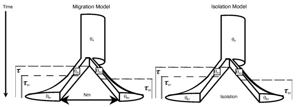
Background: MTML-msBayes uses hierarchical approximate Bayesian computation (HABC) under a coalescent model to infer temporal patterns of divergence and gene flow across codistributed taxon-pairs. Under a model of multiple codistributed taxa that diverge into taxon-pairs with subsequent gene flow or isolation, one can estimate hyper-parameters that quantify the mean and variability in divergence times or test models of migration and isolation. The software uses multi-locus DNA sequence data collected from multiple taxon-pairs and allows variation across taxa in demographic parameters as well as heterogeneity in DNA mutation rates across loci. The method also allows a flexible sampling scheme: different numbers of loci of varying length can be sampled from different taxon-pairs.

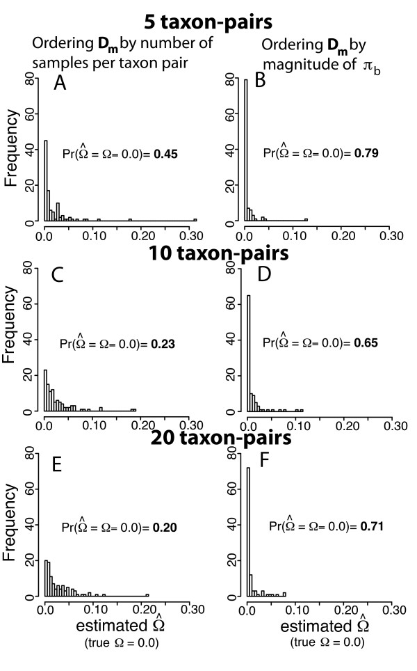
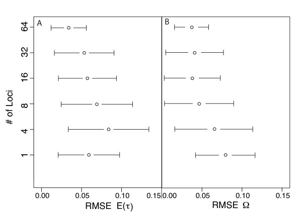
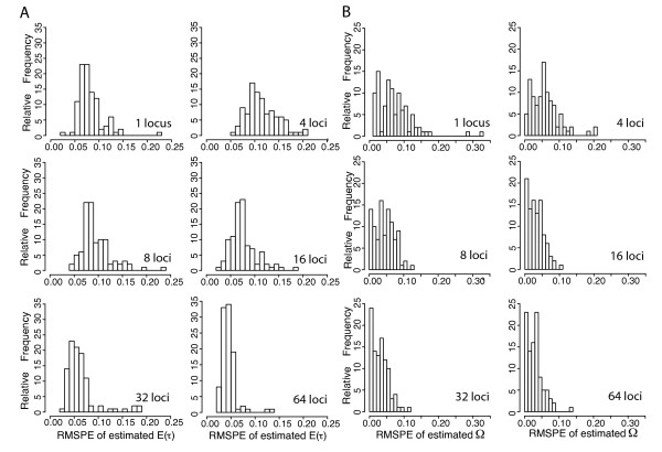
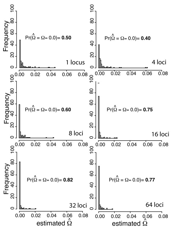
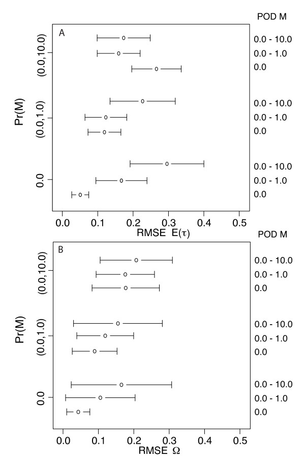
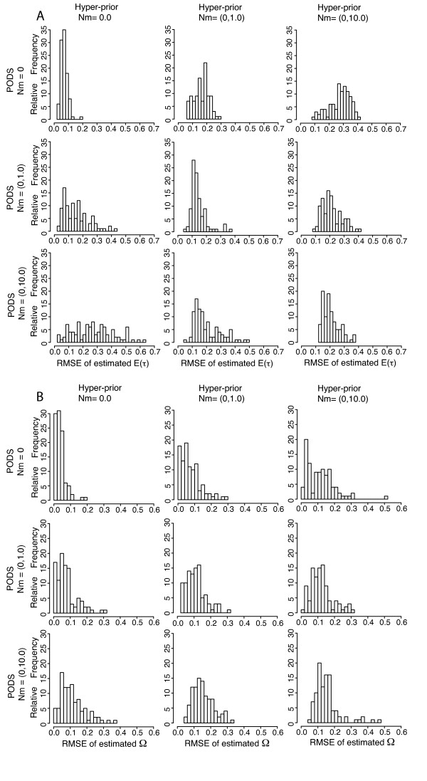
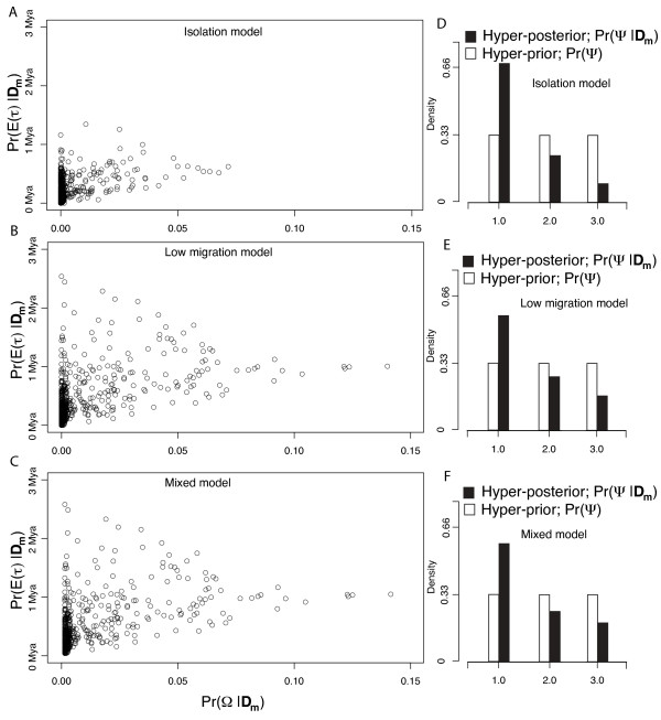
Results: Simulation tests reveal increasing power with increasing numbers of loci when attempting to distinguish temporal congruence from incongruence in divergence times across taxon-pairs. These results are robust to DNA mutation rate heterogeneity. Estimating mean divergence times and testing simultaneous divergence was less accurate with migration, but improved if one specified the correct migration model. Simulation validation tests demonstrated that one can detect the correct migration or isolation model with high probability, and that this HABC model testing procedure was greatly improved by incorporating a summary statistic originally developed for this task (Wakeley's ΨW). The method is applied to an empirical data set of three Australian avian taxon-pairs and a result of simultaneous divergence with some subsequent gene flow is inferred.

Conclusions: To retain flexibility and compatibility with existing bioinformatics tools, MTML-msBayes is a pipeline software package consisting of Perl, C and R programs that are executed via the command line. Source code and binaries are available for download at http://msbayes.sourceforge.net/ under an open source license (GNU Public License).


Figures

Figure 1
Figure 1
Depiction of isolation and migration models of a taxon diverging into sister taxa. Up to Y taxon-pairs diverge at 1 to Ψ different divergence times where all parameters shown are free to vary across the Y taxon-pairs. Additional file 1 summarizes all the parameters in the multi-taxon-pair model of divergence used in MTML-msBayes.
Figure 2
Figure 2
Comparison of sorting algorithms for summary statistic vector Dm. Frequency histograms depicting sets of 100 ABC estimates of Ω given PODS simulated under simultaneous divergence (Ω = 0; Ψ = 1) using two different algorithms for ordering the taxon-pair elements of y within Dm (panels A, C, and E by number of samples per taxon-pair; panels B, D, and F by the magnitude of the mean value of πb across loci). Results are presented for data sets that correspond to 5, 10 and 20 taxon-pairs. Each point estimate is the mode of 500 accepted points in total out of 1,500,000 simulated data sets using ABC with local linear regression.
Figure 3
Figure 3
RMSE: ABC algorithm validation for estimator bias and precision. RMSE (root mean square error) across 100 estimates of parameter values given 100 PODS (pseudo observed data sets) simulated with known parameter values. Panel A corresponds to estimates of E(τ) and panel B corresponds to estimates of Ω. The error bars depict 2 × SD (standard deviation) of the RMSE across each set of 100 estimates. For all PODS, Ψ (number divergence times across five taxon-pairs) is drawn from its discrete uniform hyper-prior ranging between 1 (simultaneous divergence) and 5 (the number of taxon-pairs). PODS and corresponding priors were simulated given data from 1, 4, 8, 16, 32 and 64 loci each from 5 taxon-pairs. Each RMSE is calculated from the 100 true hyper-parameter values (E(τ) and Ω) and the corresponding 100 posterior mode estimates (mode from the 500 accepted points out of a total 1,500,000 draws from the hyper-prior using ABC with local linear regression and a summary statistic vector Dm that only included mean values of πb across loci from every taxon-pair).
Figure 4
Figure 4
RMSPE: ABC algorithm validation for estimator bias and precision. Histograms depicting the distribution of RMSPE (root mean square posterior error) for 100 estimates of parameter values given 100 PODS (pseudo observed data sets) simulated with known parameter values. Panel A corresponds to estimates of E(τ) and panel B corresponds to estimates of Ω. For all PODS, Ψ (number divergence times across five taxon-pairs) is drawn from its discrete uniform hyper-prior ranging between 1 (simultaneous divergence) and 5 (the number of taxon-pairs). PODS and corresponding priors were simulated given data from 1, 4, 8, 16, 32 and 64 loci each from 5 taxon-pairs. Each RMSPE is calculated from the true hyper-parameter value (E(τ) and Ω) and the corresponding 500 accepted points out of a total 1,500,000 draws from the hyper-prior using ABC with local linear regression and a summary statistic vector Dm that only included mean values of πb across loci from every taxon-pair.
Figure 5
Figure 5
ABC algorithm validation for estimator accuracy under simultaneous divergence. Frequency histograms of sets of 100 ABC estimates of E(τ) (panel A) and Ω (panel B) with each test data set simulated under simultaneous divergence (Ω = 0; Ψ = 1) and each simulated draw from the hyper-prior had the number divergence times across five taxon-pairs (Ψ) drawn from its discrete uniform hyper-prior between 1 (simultaneous divergence) and 5 (the number of taxon-pairs). Test data and corresponding priors were simulated given data from 1, 4, 8, 16, 32 and 64 loci each from 5 taxon-pairs. Each point estimate is the mode of 500 accepted points in total out of 1,500,000 simulated data sets using ABC with local linear regression and a summary statistic vector Dm that only included mean values of πb across loci from every taxon-pair.
Figure 6
Figure 6
RMSE: ABC algorithm validation given different levels of assumed and known migration rates and Dm = πb. RMSE (root mean square error) across 100 estimates of parameter values given 100 PODS (pseudo observed data sets) simulated with known parameter values. Panel A corresponds to estimates of E(τ) and panel B corresponds to estimates of Ω. The error bars depict 2 × SD (standard deviation) of the RMSE across each set of 100 estimates. For all PODS, Ψ (number divergence times across five taxon-pairs) is drawn from its discrete uniform hyper-prior ranging between 1 (simultaneous divergence) and 5 (the number of taxon-pairs). PODS and corresponding priors were simulated given 16 loci each from 5 taxon-pairs. Three different hyper-priors were used with respect to post-divergence migration rates as well with simulating PODS (migration rate Nm = 0, 0-1, and 0-10 migrants per generation where migration rate varies independently across taxon-pairs within each 5 taxon-pair data set). Each RMSE is calculated from the 100 true hyper-parameter values (E(τ) and Ω) and the corresponding 100 posterior mode estimates (mode from the 500 accepted points out of a total 1,500,000 draws from the hyper-prior using ABC with local linear regression and a summary statistic vector Dm that only included mean values of πb across loci from every taxon-pair).
Figure 7
Figure 7
RMSPE: ABC algorithm validation given different levels of assumed and known migration rates and Dm = πb. Histograms depicting the distribution of RMSPE (root mean square posterior error) for 100 estimates of parameter values given 100 PODS (pseudo observed data sets) simulated with known parameter values. Panel A corresponds to estimates of E(τ) and panel B corresponds to estimates of Ω. For all PODS, Ψ (number divergence times across five taxon-pairs) is drawn from its discrete uniform hyper-prior ranging between 1 (simultaneous divergence) and 5 (the number of taxon-pairs). PODS and corresponding priors were simulated given 16 loci each from 5 taxon-pairs. Three different hyper-priors were used with respect to post-divergence migration rates as well with simulating PODS (migration rate Nm = 0, 0-1, and 0-10 migrants per generation where migration rate varies independently across taxon-pairs within each 5 taxon-pair data set). Each RMSPE is calculated from the true hyper-parameter value (E(τ) and Ω) and the corresponding 500 accepted points out of a total 1,500,000 draws from the hyper-prior using ABC with local linear regression and a summary statistic vector Dm that only included mean values of πb across loci from every taxon-pair.
Figure 8
Figure 8
Estimates of the mean, dispersion index and number of divergence times given empirical data. Panels A, B and C depict joint posterior densities of two hyper-parameter summaries that characterize the average divergence time (E(τ)) and dispersion index of divergence times Ω = Var(τ)/E(τ)) across three avian taxon-pairs that span the Carpentarian barrier in northern Australia. Each point is from a data set simulated using parameters randomly drawn from the prior and subsequently accepted using ABC with local linear regression (500 accepted points in total out of 3,000,000 simulated data sets) and a summary statistic vector Dm that only included mean values of πb across loci from every taxon-pair. Panels D, E, and F depict hyper-prior and hyper-posterior densities of Ψ, the number of divergence times across taxon-pairs. Panels A and D results are under a model of total isolation after divergence, panels B and E results are under a model allowing for low migration after divergence, with each taxon independently having Nm = 0.0 - 1.0 between sister taxa after divergence. Panels C and F are results using a mixed model where the posterior is averaged across the two models while weighting for the relative posterior probability under the two models. Divergence times assume an average rate across loci of 5.0 × 10⁻⁹ per site per generation and two year generation times.

Similar articles

Cited by

References

    1. Bermingham E, Moritz C. Comparative phylogeography: concepts and applications. Mol Ecol. 1998;7:367–369. doi: 10.1046/j.1365-294x.1998.00424.x. - DOI
    1. Arbogast BS, Kenagy GJ. Comparative phylogeography as an integrative approach to historical biogeography. J Biogeogr. 2001;28:819–825. doi: 10.1046/j.1365-2699.2001.00594.x. - DOI
    1. Coyne JA, Orr HA. Speciation. Sunderland, MA: Sinauer Associates Inc; 2004.
    1. Avise JC. Phylogeography: The history and formation of species. Cambridge: Harvard University Press; 2000.
    1. Hubbell SP. The Unified Neutral Theory of Biodiversity and Biogeography. Princeton, NJ: Princeton University Press; 2001.

Publication types

LinkOut - more resources