Diffeomorphic registration using geodesic shooting and Gauss-Newton optimisation

Abstract

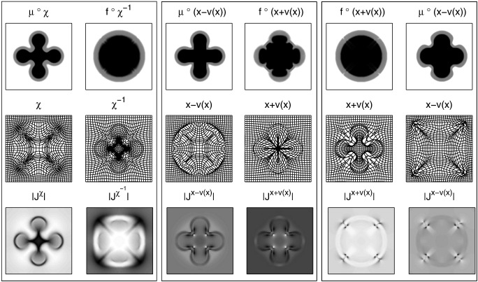
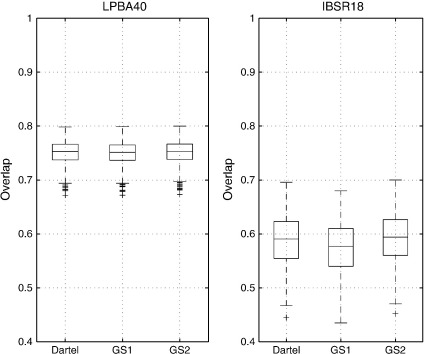
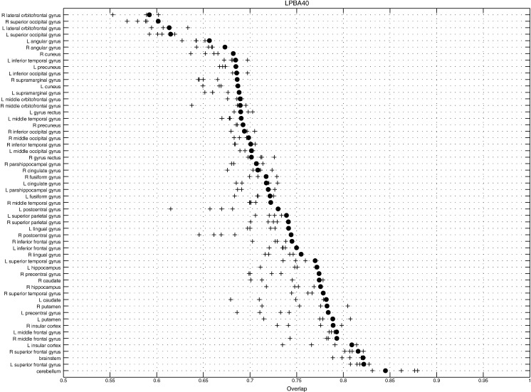
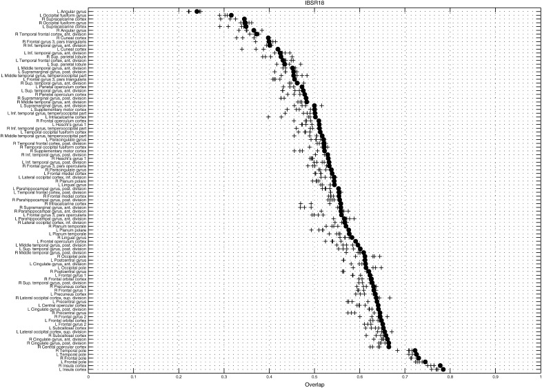
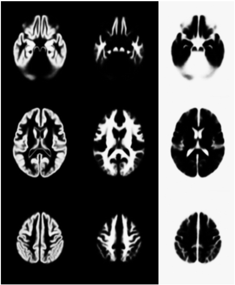
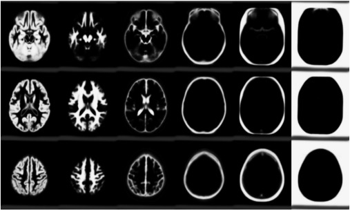
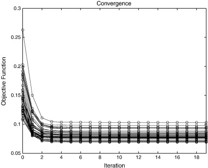
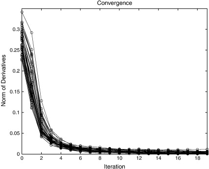
This paper presents a nonlinear image registration algorithm based on the setting of Large Deformation Diffeomorphic Metric Mapping (LDDMM), but with a more efficient optimisation scheme--both in terms of memory required and the number of iterations required to reach convergence. Rather than perform a variational optimisation on a series of velocity fields, the algorithm is formulated to use a geodesic shooting procedure, so that only an initial velocity is estimated. A Gauss-Newton optimisation strategy is used to achieve faster convergence. The algorithm was evaluated using freely available manually labelled datasets, and found to compare favourably with other inter-subject registration algorithms evaluated using the same data.

Fig. 1

The inverse of the elasticity operator, which is used for computing velocity from momentum (v_t = Ku_t). This is the Green's function (fundamental solution for a linear partial differential operator). Note that this figure shows a 2D version of the operator. Obtaining the x (horizontal) component of the velocity involves convolving the x component of the momentum with the function shown at the top left, and adding the y (vertical) component of the momentum, convolved with the function shown at the top right. Similarly, obtaining the velocity's y component is by convolving the momentum's x component with the lower-left function, and adding this to the momentum's y component convolved with the lower-right function.

Fig. 2

Results of diffeomorphic registation of two simulated images. Original images (top row), registered images (2nd row), diffeomorphic deformations (3rd row) and Jacobian determinants (bottom).

Fig. 3

Convergence of the Gauss–Newton optimisation. The top panel shows how the objective function is reduced at each iteration, whereas the lower panel shows the norm of the derivatives of the objective function with respect to the model parameters. At the exact solution (either globally or locally optimal), this norm should be zero.

Fig. 4

Illustration of the evolution equations for computing diffeomorphisms. The top row shows the system at time zero, which is followed in successive rows at later time points. Note that only eight time points were used for this integration, and that images are scaled so that intensities range between the overall minimum and maximum values within each column. Darker regions indicate larger values.

Fig. 5

Various other deformation model results. Left panel: registration using a log-Euclidean model (Eq. (33)). Centre panel: small-deformation of the template to the individual (Eq. (34)). Right panel: small-deformation of the individual to the template (Eq. (35)). Note that the Jacobian determinant images are shown scaled between their minimum and maximum values and that darker regions indicate larger values.

Fig. 6

The velocity (left panel) and “momentum” (right panel) fields of the four models. The left column shows the horizontal component, whereas the right column shows the vertical component. The top row shows the initial velocities and momenta obtained using the shooting method. Velocities and momenta from the log-Euclidean method (Eq. (33)) are shown in the second row. Those from the small-deformation methods are shown in the third (Eq. (34)) and fourth (Eq. (35)) rows.

Fig. 7

Volume overlap measures compare favourably with those obtained from the other registration algorithms evaluated in Klein et al. (2009) (this figure may be compared directly with Fig. 5 of that paper). On each box, the central mark is the median, the edges of the box are the 25th and 75th percentiles, the whiskers extend to the most extreme data-points not considered outliers. Any outliers are plotted individually.

Fig. 8

Average volume overlap for each region in the LPBA40 dataset (GS2). Results from the current GS approach are shown with filled circles. Crosses indicate results from the four algorithms evaluated in Klein et al. (2009) that performed best for this dataset (ART (Ardekani et al., 1995), SyN (Avants and Epstein, 2008), FNIRT (Andersson et al., 2007) and JRD-fluid (Chiang et al., 2007)).

Fig. 9

Average volume overlap for each region in the IBSR18 dataset (GS2). Results from the current GS approach are shown with filled circles. Crosses indicate results from the four algorithms evaluated in Klein et al. (2009) that performed best for this dataset (SPM_D (Ashburner, 2007), SyN (Avants and Epstein, 2008), IRTK (Rueckert et al., 2006) and ART (Ardekani et al., 1995)).

Fig. 10

The LPBA40 tissue probability template, showing slices 40, 60 and 80 (GS2).

Fig. 11

The IBSR tissue probability template, showing slices 40, 60 and 80 (GS2).

Fig. 12

Objective function after different numbers of Gauss-Newton iterations, when matching the images in the LPBA40 dataset to their average.

Fig. 13

The norm of the derivatives of the objective function after different numbers of Gauss–Newton iterations. In principle, the norm should be zero if the algorithm has fully converged.

Fig. 14

A single slice through the divergence of velocity fields computed after registering one of the LPBA40 subjects. The top row shows results from registering via GS, whereas the bottom row shows results from using Dartel. Results from un-translated data are shown (left column), followed by results of translated images with poor starting estimates (middle column) and finally results from translated data with close starting estimates (right column).

References

1. Andersson J.L.R., Jenkinson M., Smith S.M. FMRIB Analysis Group Technical Reports: TR07JA02. 2007. Non-linear registration, aka spatial normalisation.
1. Ardekani B.A., Braun M., Hutton B.F., Kanno I., Iida H. A fully automatic multimodality image registration algorithm. Journal of computer assisted tomography. 1995;190(4):615. - PubMed
1. Arsigny V., Commowick O., Pennec X., Ayache N. Medical Image Computing and Computer-Assisted Intervention — MICCAI 2006. 2006. A Log-Euclidean framework for statistics on diffeomorphisms; pp. 924–931. - PubMed
1. Arsigny V., Commowick O., Ayache N., Pennec X. A fast and log-Euclidean polyaffine framework for locally linear registration. Journal of Mathematical Imaging and Vision. 2009;330(2):222–238.
1. Ashburner J. A fast diffeomorphic image registration algorithm. Neuroimage. 2007;380(1):95–113. - PubMed
Publication types
LinkOut - more resources