High-Dimensional Sparse Factor Modeling: Applications in Gene Expression Genomics

Abstract

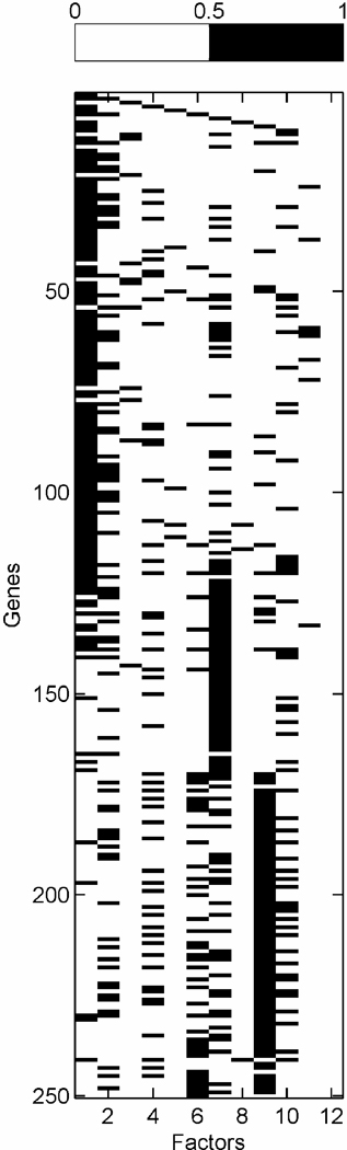
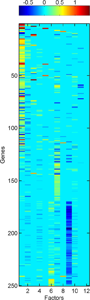
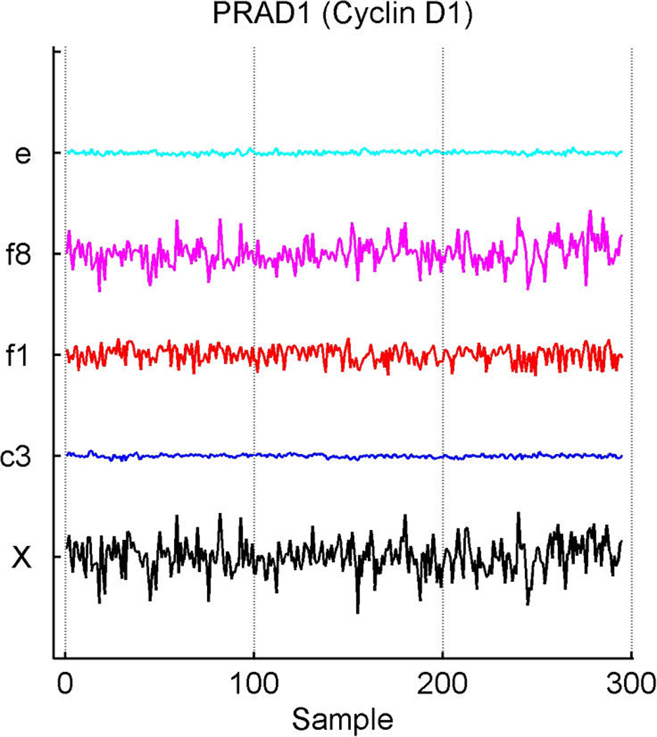
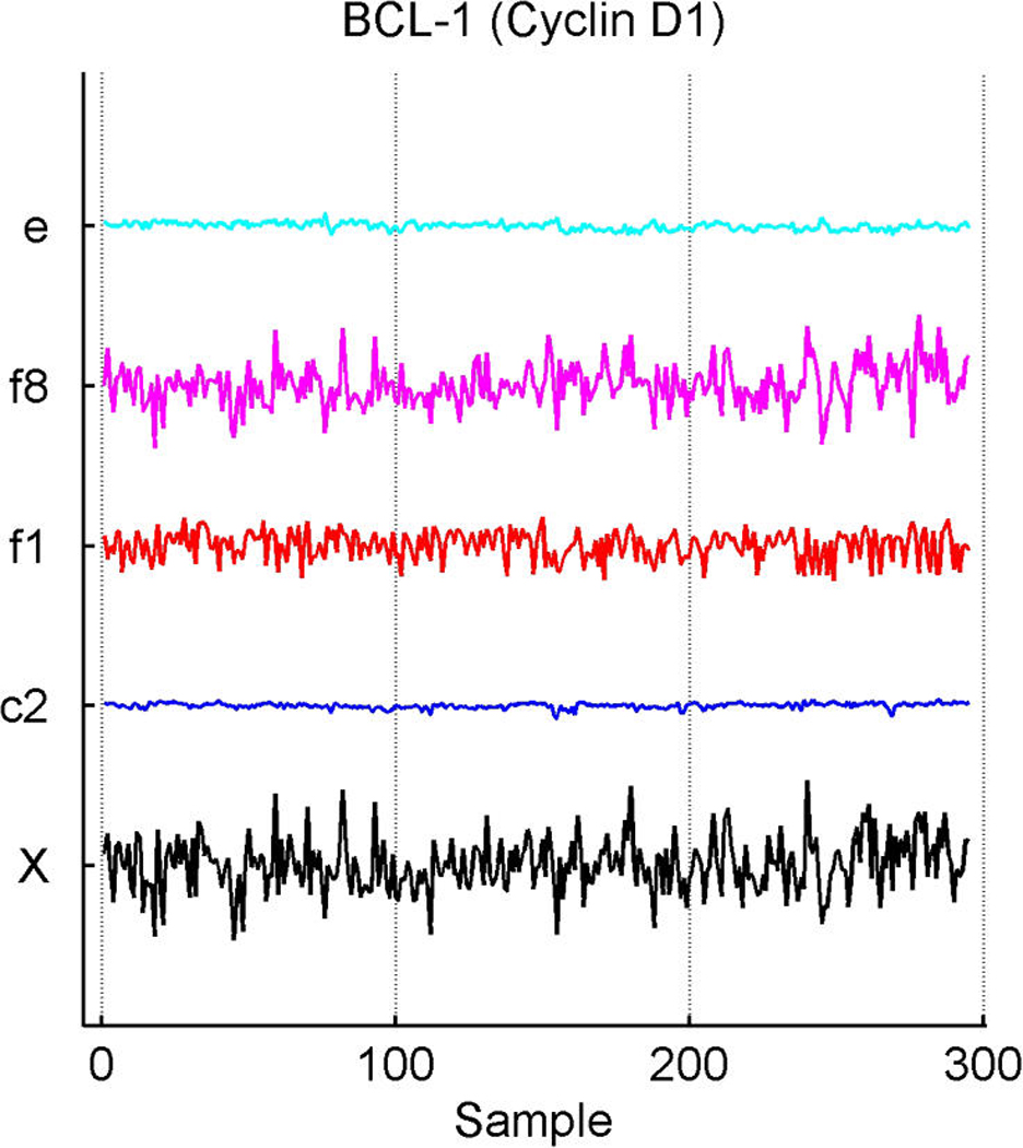
We describe studies in molecular profiling and biological pathway analysis that use sparse latent factor and regression models for microarray gene expression data. We discuss breast cancer applications and key aspects of the modeling and computational methodology. Our case studies aim to investigate and characterize heterogeneity of structure related to specific oncogenic pathways, as well as links between aggregate patterns in gene expression profiles and clinical biomarkers. Based on the metaphor of statistically derived "factors" as representing biological "subpathway" structure, we explore the decomposition of fitted sparse factor models into pathway subcomponents and investigate how these components overlay multiple aspects of known biological activity. Our methodology is based on sparsity modeling of multivariate regression, ANOVA, and latent factor models, as well as a class of models that combines all components. Hierarchical sparsity priors address questions of dimension reduction and multiple comparisons, as well as scalability of the methodology. The models include practically relevant non-Gaussian/nonparametric components for latent structure, underlying often quite complex non-Gaussianity in multivariate expression patterns. Model search and fitting are addressed through stochastic simulation and evolutionary stochastic search methods that are exemplified in the oncogenic pathway studies. Supplementary supporting material provides more details of the applications, as well as examples of the use of freely available software tools for implementing the methodology.

Figure 1

Breast cancer hormonal pathways. Skeleton of the fitted model for the 250 selected genes and 12 factors. (a) (Binary) heatmap of thresholded approximate posterior loading probabilities, I(π̂ _{g, j} > .99). (b) Heatmap of approximate posterior means of significant gene-factor loadings, α̂ _{g, j}

Figure 1

Breast cancer hormonal pathways. Skeleton of the fitted model for the 250 selected genes and 12 factors. (a) (Binary) heatmap of thresholded approximate posterior loading probabilities, I(π̂ _{g, j} > .99). (b) Heatmap of approximate posterior means of significant gene-factor loadings, α̂ _{g, j}

Figure 2

Breast cancer hormonal pathways. Plot across breast tumour samples of levels of expression (X) of the gene Cyclin D1. (a) The PRAD1/CCND1 probeset on the Affymetrix u95av2 microarray, one of the three probe sets for cyclin D1 on this array. (b) The BCL-1/CCND1 probeset. (c) The primary CCND1 probeset. Factors labelled “f” are primary latent factors, “c” indicates assay artifact covariates, and “e” represents the fitted residuals. In each of three frames, the plotted gene expression, factor, and residual levels are on the same vertical scale within the frame, so indicating the breakdown of the expression fluctuations for cyclin D1 gene probesets according to contributions from the factors. Factor 1 is the primary ER factor, and factor 8 a factor defined by the three probesets for cyclin D1, as discussed in the text.

Figure 2

Breast cancer hormonal pathways. Plot across breast tumour samples of levels of expression (X) of the gene Cyclin D1. (a) The PRAD1/CCND1 probeset on the Affymetrix u95av2 microarray, one of the three probe sets for cyclin D1 on this array. (b) The BCL-1/CCND1 probeset. (c) The primary CCND1 probeset. Factors labelled “f” are primary latent factors, “c” indicates assay artifact covariates, and “e” represents the fitted residuals. In each of three frames, the plotted gene expression, factor, and residual levels are on the same vertical scale within the frame, so indicating the breakdown of the expression fluctuations for cyclin D1 gene probesets according to contributions from the factors. Factor 1 is the primary ER factor, and factor 8 a factor defined by the three probesets for cyclin D1, as discussed in the text.

Figure 2

Breast cancer hormonal pathways. Plot across breast tumour samples of levels of expression (X) of the gene Cyclin D1. (a) The PRAD1/CCND1 probeset on the Affymetrix u95av2 microarray, one of the three probe sets for cyclin D1 on this array. (b) The BCL-1/CCND1 probeset. (c) The primary CCND1 probeset. Factors labelled “f” are primary latent factors, “c” indicates assay artifact covariates, and “e” represents the fitted residuals. In each of three frames, the plotted gene expression, factor, and residual levels are on the same vertical scale within the frame, so indicating the breakdown of the expression fluctuations for cyclin D1 gene probesets according to contributions from the factors. Factor 1 is the primary ER factor, and factor 8 a factor defined by the three probesets for cyclin D1, as discussed in the text.

Figure 3

Breast cancer hormonal pathways. Plot across breast tumor samples of levels of expression (X) of the ER gene (a) and of the HER3 epidermal growth factor receptor tyrosine kinase (b), together with the estimates of factors contributing significantly to their expression fluctuations. Factors labelled “f” are primary latent factors, “y” indicates response factors, “c” indicates assay artifact covariates, and “e” represents the fitted residuals; other layout details are as in Figure 2. Note that f7 picks up what is clear artifact related to the different substudies generating the data, and also that some residual structure remains evident in the residual plot that appears to be batch-related (e.g., an early burst of positively correlated cases).

Figure 3

Breast cancer hormonal pathways. Plot across breast tumor samples of levels of expression (X) of the ER gene (a) and of the HER3 epidermal growth factor receptor tyrosine kinase (b), together with the estimates of factors contributing significantly to their expression fluctuations. Factors labelled “f” are primary latent factors, “y” indicates response factors, “c” indicates assay artifact covariates, and “e” represents the fitted residuals; other layout details are as in Figure 2. Note that f7 picks up what is clear artifact related to the different substudies generating the data, and also that some residual structure remains evident in the residual plot that appears to be batch-related (e.g., an early burst of positively correlated cases).

Figure 4

Breast cancer hormonal pathways. Scatterplots of the posterior means of designated ER factor 1 and HER2/ERB–B2 factor 3. Color coding indicates the global measurement of protein level from IHC assays. (a) Red, ER+; blue, ER−; cyan, missing/indeterminate. (b) Red, HER2+; blue, HER2−; cyan, missing/indeterminate.

Figure 4

Breast cancer hormonal pathways. Scatterplots of the posterior means of designated ER factor 1 and HER2/ERB–B2 factor 3. Color coding indicates the global measurement of protein level from IHC assays. (a) Red, ER+; blue, ER−; cyan, missing/indeterminate. (b) Red, HER2+; blue, HER2−; cyan, missing/indeterminate.

Figure 5

Breast cancer hormonal pathways. Scatterplots of fitted probabilities of ER+ (a) and HER2+ (b) from the overall factor regression model that includes probit components for these two binary responses. Color coding indicates hormonal receptor status; in each case, red, positive; blue, negative; magenta, missing; cyan, indeterminate.

Figure 5

Breast cancer hormonal pathways. Scatterplots of fitted probabilities of ER+ (a) and HER2+ (b) from the overall factor regression model that includes probit components for these two binary responses. Color coding indicates hormonal receptor status; in each case, red, positive; blue, negative; magenta, missing; cyan, indeterminate.

Figure 6

Breast cancer hormonal pathways. The plots display the approximate predictive density contours and observed data for two selected bivariate margins on four genes, HER2/ERB–B2 (a) and the ER-related FOXA1, TFF3, and CA12 (b), with the observed data marked as crosses.

Figure 6

Breast cancer hormonal pathways. The plots display the approximate predictive density contours and observed data for two selected bivariate margins on four genes, HER2/ERB–B2 (a) and the ER-related FOXA1, TFF3, and CA12 (b), with the observed data marked as crosses.

Figure 7

Decomposition of expression over samples of several top genes in the annotated ER factors 1 and 3 (a), cell development factor 4 (b), and immunoregulatory factor 6 (c).

Figure 7

Decomposition of expression over samples of several top genes in the annotated ER factors 1 and 3 (a), cell development factor 4 (b), and immunoregulatory factor 6 (c).

Figure 7

Decomposition of expression over samples of several top genes in the annotated ER factors 1 and 3 (a), cell development factor 4 (b), and immunoregulatory factor 6 (c).

Figure 7

Decomposition of expression over samples of several top genes in the annotated ER factors 1 and 3 (a), cell development factor 4 (b), and immunoregulatory factor 6 (c).

Figure 7

Decomposition of expression over samples of several top genes in the annotated ER factors 1 and 3 (a), cell development factor 4 (b), and immunoregulatory factor 6 (c).

Figure 7

Decomposition of expression over samples of several top genes in the annotated ER factors 1 and 3 (a), cell development factor 4 (b), and immunoregulatory factor 6 (c).

Figure 8

Breast cancer p53 study. Boxplots of fitted (a, c) and out-of-sample predicted (b, d) probabilities of p53 mutant versus wild-type (a, b) and ER positive versus negative (c, d).

Figure 8

Breast cancer p53 study. Boxplots of fitted (a, c) and out-of-sample predicted (b, d) probabilities of p53 mutant versus wild-type (a, b) and ER positive versus negative (c, d).

Figure 8

Breast cancer p53 study. Boxplots of fitted (a, c) and out-of-sample predicted (b, d) probabilities of p53 mutant versus wild-type (a, b) and ER positive versus negative (c, d).

Figure 8

Breast cancer p53 study. Boxplots of fitted (a, c) and out-of-sample predicted (b, d) probabilities of p53 mutant versus wild-type (a, b) and ER positive versus negative (c, d).

Figure 9

Breast cancer p53 study: Kaplan–Meier survival curves for the training samples (n = 201) split according to the indicated thresholds. (a) Q1 represents thresholding at the first quartile of the fitted linear predictor. (b) Q2 represents thresholding at the median. (c) Stratification simply on p53 wild-type versus mutant. (d) Stratification based on the p53 classification proposed by Miller et al. (2005).

Figure 9

Breast cancer p53 study: Kaplan–Meier survival curves for the training samples (n = 201) split according to the indicated thresholds. (a) Q1 represents thresholding at the first quartile of the fitted linear predictor. (b) Q2 represents thresholding at the median. (c) Stratification simply on p53 wild-type versus mutant. (d) Stratification based on the p53 classification proposed by Miller et al. (2005).

Figure 9

Breast cancer p53 study: Kaplan–Meier survival curves for the training samples (n = 201) split according to the indicated thresholds. (a) Q1 represents thresholding at the first quartile of the fitted linear predictor. (b) Q2 represents thresholding at the median. (c) Stratification simply on p53 wild-type versus mutant. (d) Stratification based on the p53 classification proposed by Miller et al. (2005).

Figure 9

Breast cancer p53 study: Kaplan–Meier survival curves for the training samples (n = 201) split according to the indicated thresholds. (a) Q1 represents thresholding at the first quartile of the fitted linear predictor. (b) Q2 represents thresholding at the median. (c) Stratification simply on p53 wild-type versus mutant. (d) Stratification based on the p53 classification proposed by Miller et al. (2005).

Figure 10

Breast cancer p53 study: Kaplan–Meier survival curves for the test samples (n = 50) split according to the indicated thresholds. (a) Q1 represents thresholding at the first quartile of the predicted linear predictor. (b) Q2 represents thresholding at the median. (c) Stratification simply on p53 wild-type versus mutant. (d) Stratification based on the p53 classification proposed by Miller et al. 2005.

Figure 10

Breast cancer p53 study: Kaplan–Meier survival curves for the test samples (n = 50) split according to the indicated thresholds. (a) Q1 represents thresholding at the first quartile of the predicted linear predictor. (b) Q2 represents thresholding at the median. (c) Stratification simply on p53 wild-type versus mutant. (d) Stratification based on the p53 classification proposed by Miller et al. 2005.

Figure 10

Breast cancer p53 study: Kaplan–Meier survival curves for the test samples (n = 50) split according to the indicated thresholds. (a) Q1 represents thresholding at the first quartile of the predicted linear predictor. (b) Q2 represents thresholding at the median. (c) Stratification simply on p53 wild-type versus mutant. (d) Stratification based on the p53 classification proposed by Miller et al. 2005.

Figure 10

Breast cancer p53 study: Kaplan–Meier survival curves for the test samples (n = 50) split according to the indicated thresholds. (a) Q1 represents thresholding at the first quartile of the predicted linear predictor. (b) Q2 represents thresholding at the median. (c) Stratification simply on p53 wild-type versus mutant. (d) Stratification based on the p53 classification proposed by Miller et al. 2005.

References

1. Aguilar O, West M. Bayesian Dynamic Factor Models and Portfolio Allocation. Journal of Business & Economic Statistics. 2000;18:338–357.
1. Albert J, Johnson V. Ordinal Data Models. New York: Springer-Verlag; 1999.
1. Broet P, Richardson S, Radvanyi F. Bayesian Hierarchical Model for Identifying Changes in Gene Expression From Microarray Experiments. Journal of Computational Biology. 2002;9:671–683. - PubMed
1. Carvalho C. unpublished doctoral thesis. Duke University, ISDS; 2006. Structure and Sparsity in High-Dimensional Multivariate Analysis. available at http://stat.duke.edu/people/theses/carlos.html.
1. Clyde M, George E. Model Uncertainty. Statistical Science. 2004;19:81–94.
Publication types