Spatiotemporal analysis of multichannel EEG: CARTOOL

Abstract

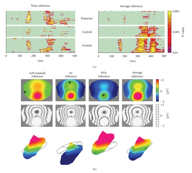
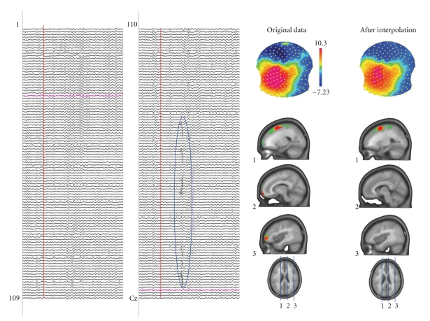
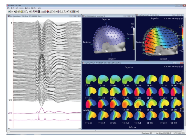
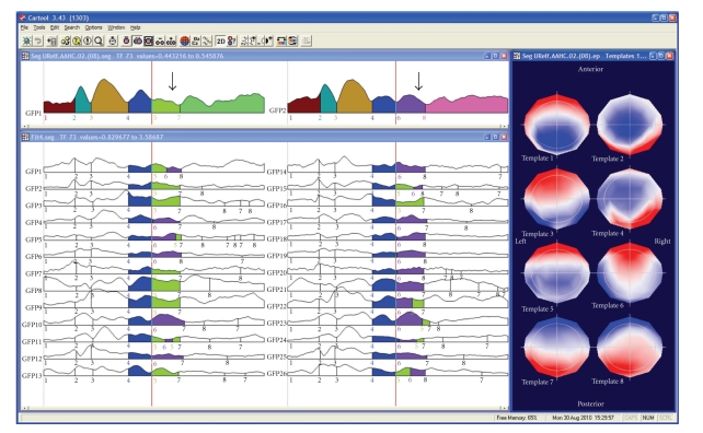
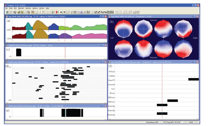
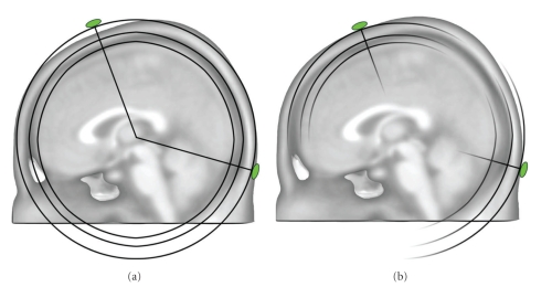
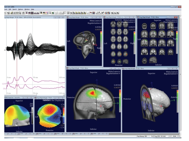
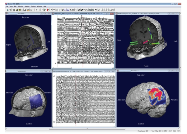
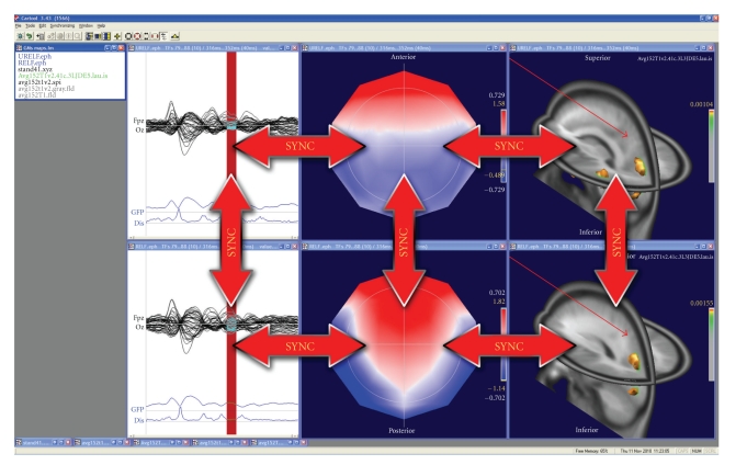
This paper describes methods to analyze the brain's electric fields recorded with multichannel Electroencephalogram (EEG) and demonstrates their implementation in the software CARTOOL. It focuses on the analysis of the spatial properties of these fields and on quantitative assessment of changes of field topographies across time, experimental conditions, or populations. Topographic analyses are advantageous because they are reference independents and thus render statistically unambiguous results. Neurophysiologically, differences in topography directly indicate changes in the configuration of the active neuronal sources in the brain. We describe global measures of field strength and field similarities, temporal segmentation based on topographic variations, topographic analysis in the frequency domain, topographic statistical analysis, and source imaging based on distributed inverse solutions. All analysis methods are implemented in a freely available academic software package called CARTOOL. Besides providing these analysis tools, CARTOOL is particularly designed to visualize the data and the analysis results using 3-dimensional display routines that allow rapid manipulation and animation of 3D images. CARTOOL therefore is a helpful tool for researchers as well as for clinicians to interpret multichannel EEG and evoked potentials in a global, comprehensive, and unambiguous way.

Figure 1

The reference issue in EEG: EEG waveform analysis is reference-dependent while topographical analysis is not. (a) Statistical comparison of evoked potential waveforms of two conditions (illusory contours versus no contours from [10]) for each electrode and each time point. Left: All electrodes referenced to the nose, right: all electrodes referenced to the Average Reference. Note the change of the results in time as well as in space. (b) Scalp potential map (seen from top) referenced to different electrodes. Top: color maps. Middle: same maps displayed with isopotential lines. Bottom: same maps displayed in relief with the zero level indicated. Note that the topography of the maps does not change, only the zero line and thus the color codes change.

Figure 2

Artifact detection by inspecting the potential maps. The left panel shows spontaneous EEG recorded from 204 electrodes. Some artifacts, like the one encircled, are easy to see in the traces and such epochs can be eliminated. However, other artifacts are not easy to see in the traces but are readily detected in the maps by isolated “islands” of potential of a certain electrode. In this example a mid-frontal and a right frontal electrode are artifact contaminated. They generate steep gradients in the electric field and consequently produce strong sources in the inverse solution (here LAURA). Interpolating these electrodes using spline interpolation eliminates the bad electrodes and the sources caused by these artifacts disappear.

Figure 3

Example of a basic display window in CARTOOL. The individual tracks are displayed together with the Global Field Power and the Global Map Dissimilarity on the left. Tracks can also be displayed in 3D on the head surface as shown on the top right. Electrode positions and maps can be displayed in 3D or 2D. Maps can be shown at a single time point at cursor position, as animation over time or as time series of maps within a selected window.

Figure 4

Illustration of the microstate segmentation in CARTOOL. The two windows on the top show the segments resulting from the k-means cluster analysis of the grand-mean ERP of two conditions. The segments are marked under the Global Field Power curves. Different colors indicate different segments. The cluster maps of these segments are displayed on the right. Note that in the beginning the same segments are found for the two conditions, while different segments explain the later components. Fitting the cluster maps to each single subject ERP statistically tests this finding. This is illustrated here by showing that more subjects have map number 5 (green) in condition 1 and map number 6 (purple) in condition 2. Duration, explained variance and other parameters are computed for each segment and can then be statistically compared using CARTOOL or any other statistical package.

Figure 5

Illustration of the statistical analysis in CARTOOL. The same data as in Figure 2 are used and the segmentation result and the maps of the eight microstates (labeled consecutively) are again shown in the window on the top. The second window on the left shows the test of the Global Field Power (GFP). Black bars indicate time points with P < .05. The third window on the left shows the t-test for each electrode and each time point. The bottom window shows the test of topographic differences using the TANOVA method. Finally, the window on the right shows the different parameters from the map fitting methods, showing which segments have significant differences in subjects. Note that in this case the topographic analysis corresponds to the two time periods that were significant in the complex electrode-wise t-tests, while the GFP test reveals an early effect that was not significant at the single electrode level.

Figure 6

Illustration of the two head models used for the inverse solution calculation in CARTOOL. The SMAC model (a) uses 3-shell of constant radiuses for the scalp and skull, which is in average a good approximation, but can be locally inaccurate for some electrodes. Due to the spherization step, the geometrical relationship between the inverse space and the electrodes is also slightly incorrect. The LSMAC model (b) uses the local radiuses of the scalp and skull, under each electrode locus, to generate different sets of 3 shells spherical model. Therefore, the forward problem is geometrically correct for each electrode.

Figure 7

Examples of displays of the source localization results in CARTOOL. The data show a grand-mean somatosensory evoked potential after left median nerve stimulation. Overlapped waveforms and the map at 20 ms are displayed on the left. The right windows show different types of displays of the sources at this time point.

Figure 8

Illustration of the display of intracranial recordings using CARTOOL. Top: recordings from depth electrodes: Left: display of the electrode positions. Middle: waveform display of the beginning of a seizure. Right: potential mapped on the electrodes. Bottom: recordings from a 8 × 8 subdural grid. Left: display of the grid position on the patient's MRI. Middle: Traces from the 64 electrodes. Right: potential mapped on the grid for one moment in time.

Figure 9

Illustration of the synchronization of windows in CARTOOL. Synchronization within the same dataset allows dynamic animations in time. Synchronization across datasets allows comparison of different conditions in time and in space.

References

1. Nunez PL, Srinivasan R. Electric Fields of the Brain: The Neurophysics of EEG. 2nd edition. New York, NY, USA: Oxford University Press; 2006.
1. Vaughan HG. The neural origins of human event-related potentials. Annals of the New York Academy of Sciences. 1982;388:125–138. - PubMed
1. Michel CM, Murray MM, Lantz G, Gonzalez S, Spinelli L, Grave De Peralta R. EEG source imaging. Clinical Neurophysiology. 2004;115(10):2195–2222. - PubMed
1. Geselowitz DB. The zero of potential. IEEE Engineering in Medicine and Biology Magazine. 1998;17(1):128–136. - PubMed
1. Lehmann D, Skrandies W. Reference-free identification of components of checkerboard-evoked multichannel potential fields. Electroencephalography and Clinical Neurophysiology. 1980;48(6):609–621. - PubMed
Publication types
LinkOut - more resources