Using the structure of inhibitory networks to unravel mechanisms of spatiotemporal patterning

Abstract

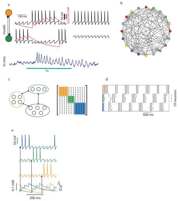
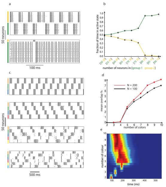
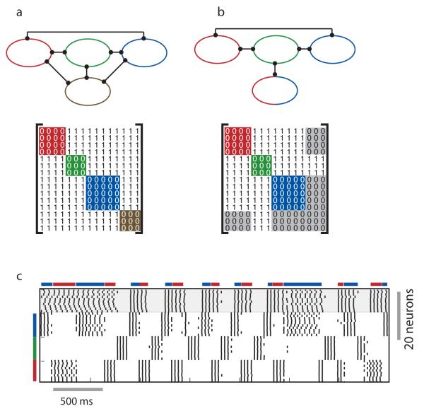
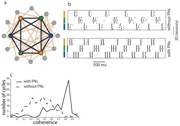
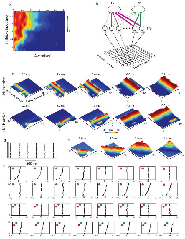
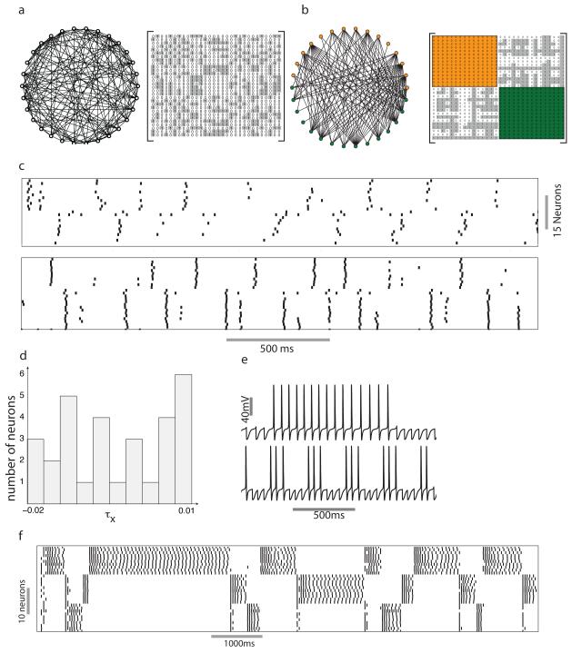
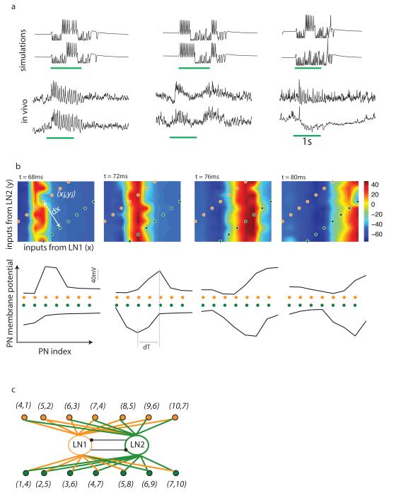
Neuronal networks exhibit a rich dynamical repertoire, a consequence of both the intrinsic properties of neurons and the structure of the network. It has been hypothesized that inhibitory interneurons corral principal neurons into transiently synchronous ensembles that encode sensory information and subserve behavior. How does the structure of the inhibitory network facilitate such spatiotemporal patterning? We established a relationship between an important structural property of a network, its colorings, and the dynamics it constrains. Using a model of the insect antennal lobe, we show that our description allows the explicit identification of the groups of inhibitory interneurons that switch, during odor stimulation, between activity and quiescence in a coordinated manner determined by features of the network structure. This description optimally matches the perspective of the downstream neurons looking for synchrony in ensembles of presynaptic cells and allows a low-dimensional description of seemingly complex high-dimensional network activity.

Figure 1

Clustering in inhibitory networks as a function of graph coloring. a) A reciprocally connected pair of inhibitory neurons is an example of a graph with chromatic number two. Left traces: An alternating pattern of bursts is generated in response to a constant external stimulus to both neurons. A Ca²⁺ dependent K current (shown in red) causes spike frequency adaptation. Right traces: In the absence of a Ca²⁺ dependent K current only one neuron produces spikes and the other is quiescent. Blue trace at the bottom: spike frequency adaptation in a local inhibitory interneuron recorded in vivo from locust antennal lobe. b) A coloring generated for a random network of 20 neurons with connection probability 0.5. c) A graph with chromatic number 3 and its corresponding adjacency matrix. d) Raster plot showing the activity of a network of 30 neurons with chromatic number three. Ten neurons are associated with each color. e) The role of Ca²⁺ concentration on the timing of LN bursts. The bottom traces show the Ca²⁺ concentration in three LNs (top three traces) associated with three different colors. The neuron with the lowest concentration of Ca²⁺ tends to spike first.

Figure 2

Dynamical properties of networks based on graph coloring. a-b) Influence of the number of neurons associated with a particular color in a network with chromatic number 2. In symmetrical networks (each group has the same number of neurons) both groups spend equal time in the active state (top panel of (a) and the point [50 50] in (b)). As the asymmetry in network structure increases, the larger group increasingly dominates ((b) and bottom panel of (a)). c-e) Influence of the number of colors. As the number of colors increased the switching pattern became more noisy (compare top and bottom panels of (c)). d) Mean overlap time for networks consisting of 100 or 200 neurons. The percentage of time during which multiple groups are simultaneously active increases with chromatic number. e) Burst length distribution as a function of chromatic number. The width of the distribution increased abruptly when the chromatic number of the graph exceeded 4.

Figure 3

Networks can have unique or multiple colorings. a) A network with a chromatic number 4 and a single coloring; b) A network with a chromatic number 3 and 2 different colorings. The neuron that may be colored either red or blue is shown with both colors. Bottom panels: adjacency matrices corresponding to the networks above. c) The dynamics of a network of 40 neurons with connectivity like the network in (b). The bars on the side of the panel correspond to the red, green and blue groups of 10 neurons. Note that the neuron colored red or blue switches allegiance between the red and the blue groups. The bars on top of the panel indicate the intervals of time when this group of neurons synchronizes with the red or the blue groups.

Figure 4

Excitation preserves coloring–based dynamics.a) Schematic of the antennal lobe network. Nodes with solid colors: groups of inhibitory interneurons associated with a particular color. Projection neurons (shown as checkered circles) are randomly connected to and receive connections from the inhibitory sub– network. b) Raster plot showing the dynamics of the inhibitory sub–network when excitatory neurons were present (bottom panel) or absent (top panel). c) The distribution of a measure of spike coherence over cycles of the local field potential oscillation, the mean coherence of spikes within a cycle increased when excitatory connections were added. The coherence (R) of spikes within each cycle of the oscillatory local field potential R_j =(∑Cosθ_i )² +(∑Sinθ_i )² was calculated for each cycle j. The distribution was generated from all values of R_j. Excitation enhanced coloring–based dynamics of the inhibitory network.

Figure 5

Coloring based reordering generates low–dimensional dynamics. a) Distribution of spikes within each cycle of the oscillatory local field potential as a function of pre–synaptic inhibitory input. For each interval of pre–synaptic inhibitory input (0.5nA intervals) neurons that produce spikes within a particular cycle were picked and the deviation of spike phase from the mean was calculated. The spread of the distribution narrowed as the inhibitory input increased (from top to bottom). b) Projection neurons were ordered in a two–dimensional space depending on the number of inputs each received from a particular group of inhibitory neurons. c) Projection neuron spikes form traveling waves in the reconstructed space. Top panel shows the activity when LN1 is active and the middle panel shows the activity when LN2 is active. d) Raster plot of LN activity when interactions between LN1 and LN2 were removed. e) The pattern of wave propagation by PNs in the network with no lateral inhibition between LNs. f) Spike raster showing the activity of a subset of neurons as a function of the phase of the oscillatory LFP. Different panels in each row correspond to different cycles of the oscillation. The color of the filled circle indicates which of the two groups of neurons (LN1 or LN2) was active during that particular cycle. Top two rows – intact LN1-LN2 inhibition. The top row of panels shows the activity of a group of neurons that receive exactly seven inputs from LN1. The second row shows a group of neurons that receive seven inputs from LN2. Bottom two rows - LN1 and LN2 are disconnected. The third row shows the activity of a group of neurons that are arranged along the diagonal of the grid. Each neuron along this diagonal receives a sum of five inputs from the groups LN1 and LN2. The fourth row shows the same group of neurons as in second row but with no LN1-LN2 inhibition.

Figure 6

Coloring–based dynamics in realistic neural networks. a) A random bipartite graph. Individual neurons receive between 1 and 14 inputs from LNs belonging to a different color and the corresponding adjacency matrix. b) The neurons were grouped into two groups based on the color. Adjacency matrix of the network shows off–diagonal blocks with ones (shaded gray) and zeros. c) Raster plot showing the response of the network to input in the absence (top panel) and the presence (bottom panel) of random excitatory input from PNs. d) Distribution of the parameter τ_x that perturbs the time scale of the Ca²⁺ dependent potassium current. e) Dynamics of inhibitory LNs as a function of τ_x. The top trace shows the response of a neuron belonging to a reciprocally inhibitory pair with τ_x = 0.01. The bottom trace shows the response of a neuron with τ_x = 0.02. f) Dynamics of a group of 30 LNs that form a three–color network. The value of τ_x for each LN in the network was picked from the distributions shown in (d).

Figure 7

a) Example traces of local inhibitory interneuron activity from model simulations (top two traces) and in vivo intra–cellular recordings from locust local interneurons (bottom two traces). In the left and central panel, traces show responses of a single LN to multiple presentations of the same odor. In the rightmost panel, the two traces show the responses of different neurons to the same odor. The green lines below the traces show the duration over which the stimulus was presented. b-c) Coloring based model of a segmental swimming pattern generator. Two groups of neurons along off–diagonal lines in the plot (b, top panels) were picked. The perpendicular distance between them is marked dx. Waves of activity generated by the network (b, top panels) were seen in these sub–groups of neurons (b, bottom panels). The time difference between the peaks of the traveling waves is marked dT. The sub–network that generates traveling waves along these lines of neurons is shown in (c). Each neuron is marked by two coordinates (x_i,y_i). The x–coordinate shows the number of inhibitory inputs received by a given PN from the group LN1. The y–coordinate shows the number of inhibitory inputs received from the group LN2.

References

1. Abeles M, Bergman H, Margalit E, Vaadia E. Spatiotemporal firing patterns in the frontal cortex of behaving monkeys. J Neurophysiol. 1993;70:1629–1638. - PubMed
1. Ahn S, Smith BH, Borisyuk A, Terman D. Analyzing Neuronal Networks Using Discrete-Time Dynamics. Physica D. 2010;239:515–528. - PMC - PubMed
1. Appel K, Haken W. Every planar map is four colorable. Illinois Journal of Mathematics. 1977a;21:439–567.
1. Appel K, Haken W. Solution of the four color map problem. Scientific American. 1977b;237:108–121.
1. Arenas A, Diaz-Guilera A, Kurths J, Moreno Y, Zhou C. Synchronization in complex networks. Physics Reports. 2008;469:93–153.
Publication types
LinkOut - more resources