Nonrenewal spike train statistics: causes and functional consequences on neural coding

Abstract

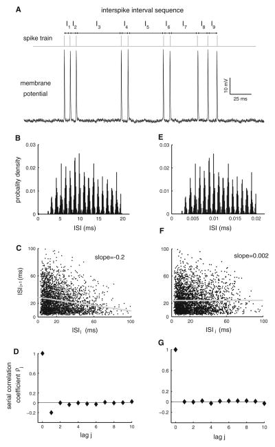
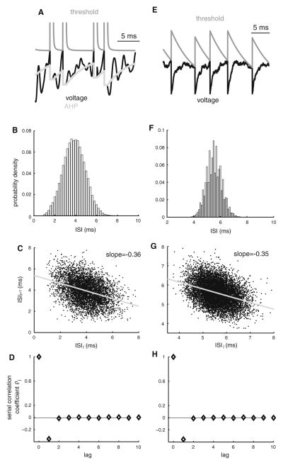
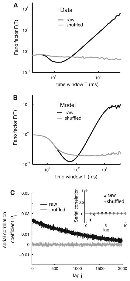
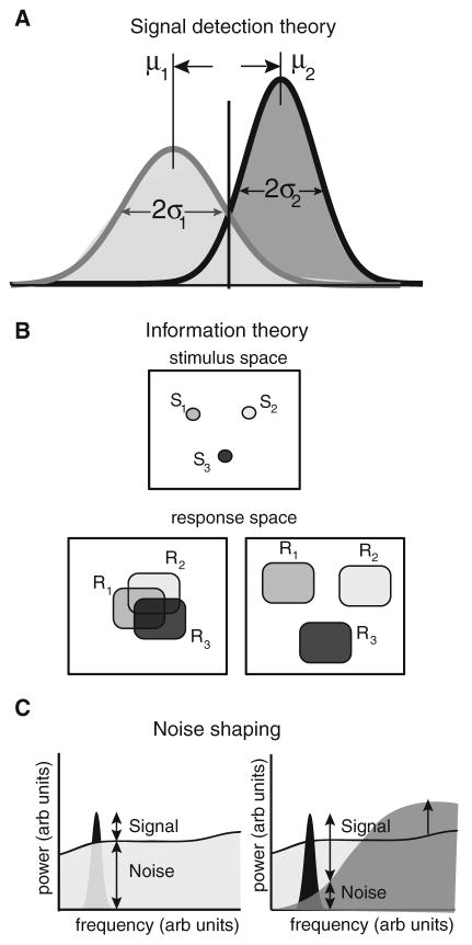
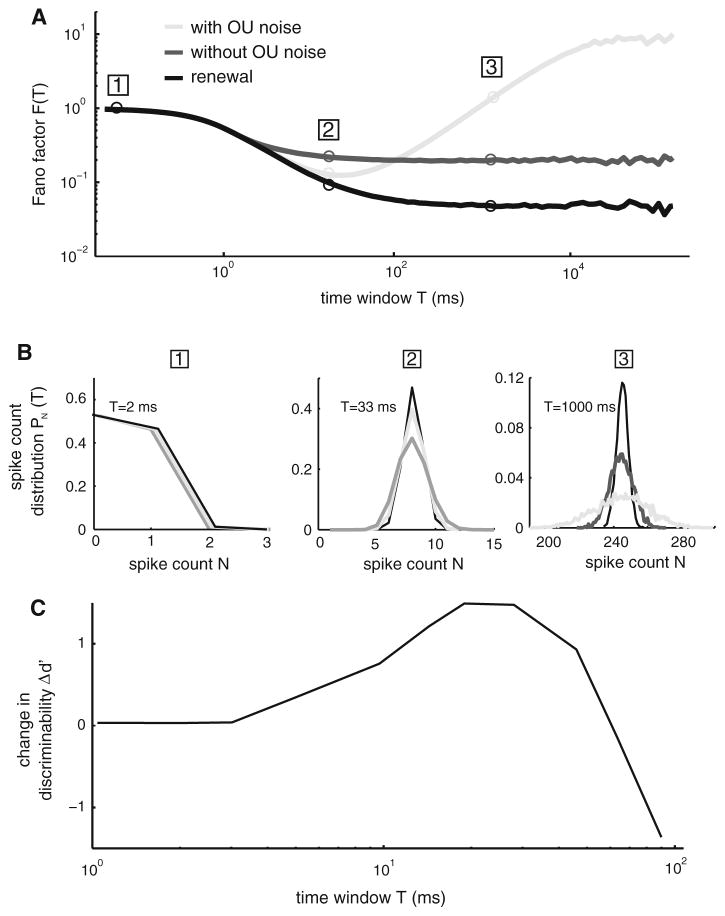
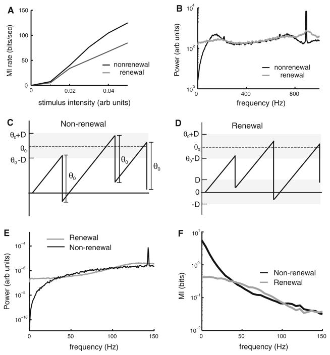
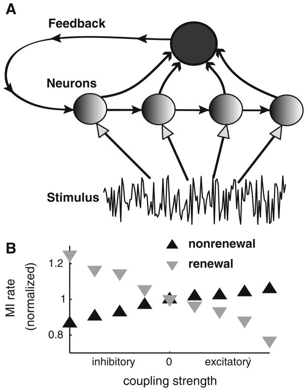
Many neurons display significant patterning in their spike trains (e.g. oscillations, bursting), and there is accumulating evidence that information is contained in these patterns. In many cases, this patterning is caused by intrinsic mechanisms rather than external signals. In this review, we focus on spiking activity that displays nonrenewal statistics (i.e. memory that persists from one firing to the next). Such statistics are seen in both peripheral and central neurons and appear to be ubiquitous in the CNS. We review the principal mechanisms that can give rise to nonrenewal spike train statistics. These are separated into intrinsic mechanisms such as relative refractoriness and network mechanisms such as coupling with delayed inhibitory feedback. Next, we focus on the functional roles for nonrenewal spike train statistics. These can either increase or decrease information transmission. We also focus on how such statistics can give rise to an optimal integration timescale at which spike train variability is minimal and how this might be exploited by sensory systems to maximize the detection of weak signals. We finish by pointing out some interesting future directions for research in this area. In particular, we explore the interesting possibility that synaptic dynamics might be matched with the nonrenewal spiking statistics of presynaptic spike trains in order to further improve information transmission.

Fig. 1

Example of nonrenewal spike train statistics. a Voltage trace from a pyramidal cell of weakly electric fish. The spike times and ISIs (I₁,… I₉) are also shown. It is seen that short ISIs tend to be followed by long ones and vice versa. b ISI probability distribution obtained from the same cell. c ISI return map obtained from the same cell. The slope of the best-fit line (gray) is equal to the ISI serial correlation coefficient at lag one for the spike train. d ISI serial correlation coefficients ρ_j as a function of lag j. Note that we have ρ₁ < 0. e The ISI probability distribution obtained after randomly shuffling the ISI sequence. f The ISI return map is significantly altered by the shuffling procedure. g ISI serial correlation coefficients ρ_j as a function of lag j for the shuffled data. Note that ρ_j = 0 for j > 0

Fig. 2

Mechanisms that give rise to nonrenewal spike train statistics. a Voltage (black) and threshold (dark gray) traces from the model proposed by Geisler and Goldberg (1966). An action potential is said to occur when the voltage is equal to the threshold. Immediately after, the threshold is set to infinity during the duration of the absolute refractory period and decreases back to its steady-state value. The voltage is the sum of noise and a variable (light gray) that is decremented immediately after an action potential. When two or more action potentials occur in rapid succession, there is a cumulative decrease in the voltage. c ISI probability distribution from this model. The ISI return map displays a negative slope (gray). d ISI serial correlation coefficients ρ_j as a function of lag j. Note that we have ρ₁ < 0. e Voltage (black) and threshold (gray) traces from the leaky integrate-and-fire model with dynamic threshold (LIFDT). Like in the Geisler–Goldberg model, an action potential is said to occur when the voltage is equal to the threshold. Immediately after, the voltage is reset to a constant (zero in this case) and the threshold is incremented by a constant amount after which it decays exponentially to a steady-state value. Repetitive firing can lead to accumulation in the threshold, causing it to be higher. We refer to this phenomenon as threshold fatigue. f ISI probability density for the LIFDT model. g The ISI return map for the LIFDT model also shows a negative slope. h ISI serial correlation coefficients ρ_j as a function of lag j for the LIFDT model. Note that we have ρ₁ < 0

Fig. 3

Detecting positive ISI correlations in experimental data and models. a Fano factor F(T) (variance to mean ratio of the spike count distribution in a time window of length T) as a function of T for an electroreceptor afferent neuron of weakly electric fish. In particular, F(T) increases as a power law for large T as can be seen from the linear part of the graph (note the log–log scale). Also shown is the Fano factor computed from the data after randomly shuffling the ISI sequence (gray) which does not display this power law behavior. b The Fano factor F(T) as a function of T for an LIFDT model that is driven by a weak noise with a long correlation time (black) resembles that obtained from the experimental data. The Fano factor F(T) obtained after shuffling the ISIs is also shown (gray). c ISI serial correlation coefficients ρ_j as a function of lag j (black) and after random ISI shuffling (gray). It is seen that the model displays weak positive ISI correlations that decay slowly over thousands of lags. Random ISI shuffling eliminates these correlations (gray). The inset shows the ISI serial correlation coefficients ρ_j as a function of lag j but only for the first 10 lags, thus showing the negative serial correlation at lag 1 and that these positive ISI correlations can be easily missed because they are so weak in magnitude

Fig. 4

Illustration of signal detection theory, information theory, and noise shaping. a Illustrating signal detection theory. The basic premise is that two different stimuli (1 and 2) will elicit two different response distributions with means μ₁, μ₂ and standard deviations σ₁, σ₂, respectively. The degree of separability between the two distributions can be assessed by computing d′. b Illustrating information theory. Information theory can be seen as a generalization of signal detection theory for more than 2 stimuli. It is assumed that different stimuli (S₁, S₂, S₃) will elicit different response distributions (R₁, R₂, R₃). If these have considerable overlap (bottom left panel), it is more difficult to know whether a given response was elicited by a given stimulus. In contrast, when these response distributions have no overlap, it then becomes easy to gain information as to which stimulus was presented when observing a given response. c Illustrating noise shaping. Shown are the power spectra of a signal (black) and the noise (gray). The signal-to-noise ratio (SNR) is then simply the ratio of signal and noise power and depends on frequency. If the noise power is high, then the signal-to-noise ratio is low (left). However, if noise power was to be transferred from frequencies contained in the signal to higher frequencies, then the SNR would be increased (right). Noise shaping is precisely the transfer of noise power from one frequency range to another, thereby conserving the total noise power (i.e. the power summed overall frequencies)

Fig. 5

Positive and negative ISI correlations act to create a minimum in spike train variability for a given time window T. a Fano factor F(T) from the LIFDT neuron model driven by a weak Ornstein–Uhlenbeck (OU) noise with a long correlation time (light gray). Also shown are the Fano factor F(T) computed from the same model without the OU noise (black) and after shuffling the ISI sequence (dark gray). b Spike count distributions P_N(T) obtained for all three conditions. For T = 2 ms (left), the distributions show almost complete overlap. However, for T = 33 ms (middle), the spike count distribution obtained from the LIFDT model without OU noise (black) shows the weakest variance, followed by the distribution obtained with the model with OU noise (light gray), followed by the distribution obtained after shuffling. However, for T = 1,000 ms (right), it is the distribution obtained from the model with OU noise (light gray) that has the highest variance. c Change in discriminability measure d′ (i.e. the difference between d′ computed from the model with OU noise and d′ computed after shuffling the ISI sequence) as a function of the time window length T. It is seen that the gain in discriminability is maximal for a value of T for which the Fano factor F(T) is minimum

Fig. 6

Negative ISI correlations increase information transmission through noise shaping. a Mutual information rate as a function of stimulus intensity for nonrenewal (black) and renewal (gray) phenomenological models. These models were matched such as to have similar ISI probability densities and signal power in response to the stimulus. b Noise power spectra for nonrenewal (black) and renewal (gray) phenomenological models. It is seen that the nonrenewal model displays lower noise power at low frequencies. c Illustration of the voltage trace from a nonrenewal simplified model (black). Unlike the LIFDT or Geisler-Goldberg models, the voltage is a linear function of time and a threshold is randomly chosen from the interval [θ₀ − D; θ₀ + D]. When the voltage reaches the threshold, it is decremented by a constant amount θ₀. It can be shown that this model gives rise to a single negative ISI correlation coefficient at lag 1, similar to the LIFT model (D). Illustration of the voltage trace from a renewal simplified model (black). The voltage is still a linear function of time, and a threshold is randomly chosen from the interval [θ₀ − D; θ₀ + D]. However, when the voltage reaches the threshold, it is instead reset to a random value in the interval [− D; D]. It can be shown that this model gives rise to renewal spike train statistics. e Noise power spectra of the simplified nonrenewal (black) and renewal (gray) models. Note the similarity with b. f Mutual information rate densities computed from the nonrenewal (black) and renewal (gray) simplified models. Note that the mutual information rate density of nonrenewal model is larger than that of the renewal model for low frequencies. This demonstrates that noise shaping leads to information shaping

Fig. 7

Effects of coupling on networks of nonrenewal and renewal model neurons. a Representation of the network connectivity. Each neuron in the network receives the same stimulus. The responses of all neurons in the network are then summed, and the resulting is then fed back to all neurons with a delay as either excitatory or inhibitory input. We note that this topology is mathematically equivalent to all-to-all coupling. b Mutual information rate normalized to its value for no coupling as a function of the coupling strength (negative values mean inhibitory coupling while positive ones mean positive coupling). It is seen that coupling affects the information transmitted by networks of renewal and nonrenewal neurons in opposite ways

References

1. Abeles M. Corticonics. Cambridge University Press; Cambridge: 1991.
1. Averbeck BB, Lee D. Effects of noise correlations on information encoding and decoding. J Neurophysiol. 2006;95:3633–3644. - PubMed
1. Averbeck BB, Latham PE, Pouget A. Neural correlations, population coding and computation. Nat Rev Neurosci. 2006;7:358–366. - PubMed
1. Avila Akerberg O, Chacron MJ. Noise shaping in neural populations. Phys Rev E. 2009;79:011914. - PMC - PubMed
1. Avila Akerberg O, Chacron MJ. Noise shaping in neural populations with global delayed feedback. Math Model Nat Phenom. 2010;5:100–124. - PMC - PubMed
Publication types
LinkOut - more resources