T-wave alternans and arrhythmogenesis in cardiac diseases

Abstract

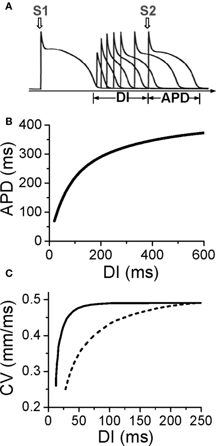
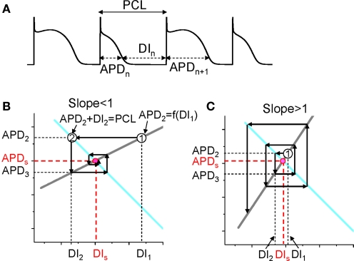
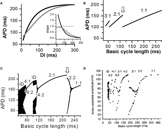
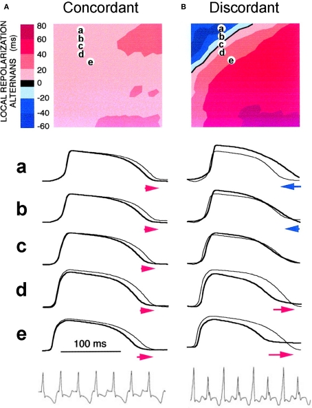
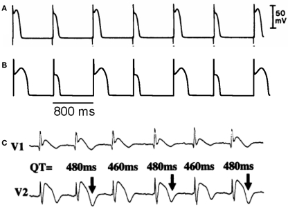
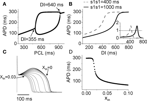
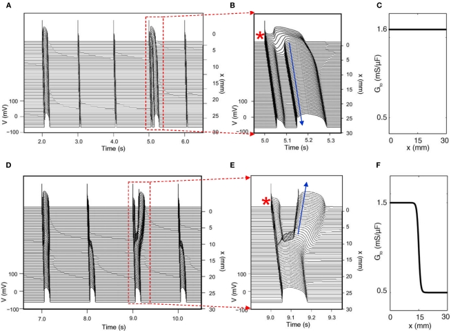
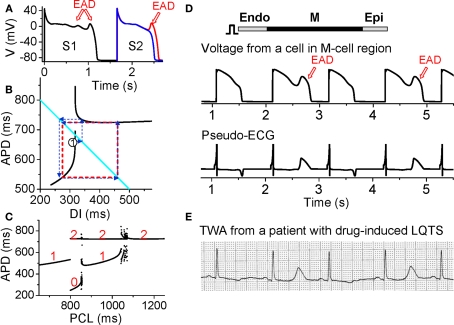
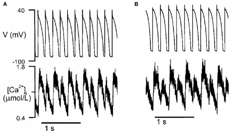
T-wave alternans, a manifestation of repolarization alternans at the cellular level, is associated with lethal cardiac arrhythmias and sudden cardiac death. At the cellular level, several mechanisms can produce repolarization alternans, including: 1) electrical restitution resulting from collective ion channel recovery, which usually occurs at fast heart rates but can also occur at normal heart rates when action potential is prolonged resulting in a short diastolic interval; 2) the transient outward current, which tends to occur at normal or slow heart rates; 3) the dynamics of early afterdepolarizations, which tends to occur during bradycardia; and 4) intracellular calcium cycling alternans through its interaction with membrane voltage. In this review, we summarize the cellular mechanisms of alternans arising from these different mechanisms, and discuss their roles in arrhythmogenesis in the setting of cardiac disease.

Keywords: T-wave alternans; afterdepolarizations; arrhythmias; calcium cycling; cardiac diseases; restitution.

Figure 1

Electrical restitution. (A) S1S2 protocol for determining APD restitution, in which the myocyte is paced with several or many beats (S1) and then a premature stimulus (S2) is given to determine the response of APD to DI. (B) An APD restitution curve (APD versus previous DI). (C). CV restitution curves (CV versus previous DI) for normal Na channel recovery (solid) and slowed Na channel recovery (dashed).

Figure 2

Dynamical instability caused by steep APD restitution curve. (A) A voltage trace illustrating the relationship between DI, APD, and PCL. (B) Cobweb diagram showing that the equilibrium point is stable when the slope of the restitution curve is smaller than one. Thick gray line is the linear APD restitution curve. The cyan line satisfying PCL = APD_n + DI_n. The intersection of these two lines is the equilibrium point at which APD = APD_s and DI = DI_s. The cobweb diagram to determine the stability was obtained as follows: starting a DI (DI₁) which is away from the equilibrium point, a vertical line intersects the APD restitution curve at point “1” which is equivalent to map DI₁ into APD₂; a horizontal line from point “1” intersects the cyan curve at a point “2” which graphically determines the next DI (DI₂); then the vertical line from point “2” intersect with the restitution curve, determining APD₃. A cobweb forms as this process continues. Note that cobweb is a standard technique to graphically track, not only the instability of an equilibrium point, but also the non-linear solutions including chaos of any iterated map. This technique can be found in any text book on non-linear dynamics and chaos, such as the one by Strogatz (2000). (C) Cobweb diagram obtained as in B showing that the equilibrium point is unstable when the slope of the APD restitution curve is greater than one. The stability of the equilibrium point can be also obtained mathematically as follows. Assume that the APD restitution curve is a linear curve described by the function APD_{n + 1} = APD_α + αDI_n. At the equilibrium point, APD_s = APD_α + αDI_s. An initial DI (DI₁) that is away from the equilibrium value DI_s (ΔDI₁ = DI₁ − DI_s) results in an APD at the next beat as APD₂ = APD_α + αDI₁ = APD_α + αDI_s + α(DI₁ − DI_s) = APD_s + αΔDI₁. Using the relationship PCL = APD_n + DI_n, one can calculate the DI (DI₂) of the next beat as DI₂ = PCL − APD₂ = PCL − (APD_s + αΔDI₁) = DI_s − αΔDI₁, and the APD (APD₃) of the following beat as APD₃ = APD_α + αDI₂ = APD_s + α(DI_s − αΔDI₁) = APD_s − α²ΔDI₁. By iterating this same process, one obtains APD of any beat as APD_n = APD_s + (−1)ⁿαⁿ⁻¹ΔDI₁. Therefore, if α < 1, αⁿΔDI₁ < αⁿ⁻¹ΔDI₁, so that APD_n becomes closer and closer to APD_s as the beat number n increases, and thus the equilibrium point is stable (as in B). If α > 1, αⁿΔDI₁ > αⁿ⁻¹ΔDI₁, so that APD_n becomes further away from APD_s as the beat number n increases, and thus the equilibrium point is unstable (as in C).

Figure 3

Action potential duration alternans and complex dynamics due to APD restitution. (A) APD restitution curves with different slope properties. Inset shows the slopes of the two APD restitution curves. (B). A bifurcation diagram by plotting APD versus PCL for the shallow APD restitution curve. The figure was obtained by iterating Eqs. 1 and 2 with many iterations for a given PCL. For each PCL, the first 100 APDs were dropped and the next 100 APDs were plotted. Since the equilibrium point is always stable, only one point for each PCL shows up on the plot in this case. However, if alternans (or chaos) occurs, two (or many) APD points will show up as is the case in C. (C) A bifurcation diagram for the steep APD restitution curve. (D) Bifurcation diagram from an experiment (Chialvo et al., 1990).

Figure 4

Spatially concordant and discordant alternans (modified from Pastore et al. (1999)). (A) Concordant alternans. Top: ΔAPD = APD_{n + 1} − APD_n distribution in space; Middle: sample action potential recordings for two consecutive beats from the sites marked on the upper panel; Bottom: Pseudo-ECG showing TWA. Since APD alternans is concordant, the color in the top panel is uniform in space (ΔAPD everywhere is positive in one beat and negative in the following beat) and since no CV restitution is engaged, no QRS alternans in the ECG. (B) Same as A but for discordant alternans. Since APD alternans is discordant, the color in the top panel is no longer uniform in space, but change from one to the other (ΔAPD changes from negative to positive as the color changes from blue to red in space, and color map reverse in the following beat), and since CV restitution is engaged, QRS alternans occurs in the ECG.

Figure 5

Action potential duration alternans induced by I_to. (A) APD alternans from a canine epicardial myocyte under “simulated ischemia” condition (Lukas and Antzelevitch, 1993). (B) APD alternans from the LR1 model with an I_to added. PCL = 800 ms which is the same as in the experiment in A. (C) ECG from a patient with Brugada syndrome showing TWA (Nishizaki et al., 2005).

Figure 6

Mechanisms of I_to induced alternans. (A) A bifurcation diagram by APD versus PCL. (B) APD restitution curves for two different S1S1 intervals. Inset shows the slopes of the two APD restitution curves. (C) Action potentials for different initial values of x (x_in = 0 to 0.03). (D) APD versus the initial values of x (x_in).

Figure 7

Phase-2 reentry due to dynamical instabilities (Modified from Maoz et al. (2009)). (A) Phase-2 reentry in a homogeneous 1D cable (I_to distribution in C). On the first beat shown, the action potential is long and exhibits spike-and-dome morphology for all cells. On the second and third beats, the action potential is short with no dome. On the fourth beat (close-up in B), however, the action potential becomes spatially heterogeneous, cells close to the pacing site (*) exhibit spike-and-dome morphology and distal cells lose the dome, leading to an anterograde phase-2 reentry (arrow). (D) Phase-2 reentry in a heterogeneous cable (I_to distribution in F). In the small I_to region, the action potential morphology is always stable, but in the large I_to region, the action potential morphology is unstable, forming retrograde phase-2 reentry on the third beat (Close-up in E).

Figure 8

Action potential duration alternans resulting from EAD dynamics. (A) S1S2 restitution protocol (as explained in Figure 1A). After the S1 beat, two S2 beats are shown in which the DI of the read trace is 1 ms larger than the blue one, showing that at the APD discontinuous point, a very small increase in DI results in an action potential with an EAD. (B) S1S2 APD restitution curve (black lines) when EADs occur at slow heart rates. The discontinuous jump in APD indicates that the action potential changes from no EAD to one EAD, or from one to two EADs, an all-or-none behavior. The cyan line satisfying PCL = APD_n + DI_n. The arrowed blue lines illustrated cobweb diagram leading to alternans (red dashed square). (C). A bifurcation diagram showing steady state APD versus PCL obtained by iterating the map as shown in B. The numbers indicate number of EADs in an action potential for the corresponding APD value. (D) Simulation results of a 1D cable showing EAD alternans and TWA. (E). ECG showing TWA from a patient with drug-induced long QT syndrome (Wegener et al., 2008). Panels A–C were modified from Sato et al., , .

Figure 9

Ca alternans in a rabbit myocyte (modified from Chudin et al. (1999)). (A) APD and Ca alternans at PCL = 180 ms. (B) Same as A but the action potential was clamped, i.e., the myocyte was paced with a fixed action potential.

Figure 10

Ca alternans from a CRU network model. (A) Ca distribution in the cytoplasmic space at the peak each beat for the six alternating beats (Rovetti et al., 2010). (B) A time–space plot (line scan) of optical signal showing Ca alternans from an experiment by Diaz et al. (2004). (C) A time–space plot of Ca from the simulation in B. The scanned line is marked in A. (D) SR depletion versus load using a “ramp pacing” by Picht et al. (2006). (E) The simulation data using a similar pacing protocol. In the simulations, the system was first paced with PCL = 500 ms for 20 beats and exhibited stable alternans (gray dots), and then increased PCL gradually (open dots), until PCL = 2000 ms at which the system exhibited regular Ca release with no alternans (black dots). For each PCL, Ca depleted from the SR was plotted against the SR Ca content right before the stimulation. In the experiment by Picht et al., the pacing frequency was decreased from 2.2 Hz (stable alternans) to 1.5 Hz (regular depletions).

Figure 11

The “3R theory” of Ca alternans. (A) A schematic plot illustrating that a CRU has primary sparking probability α, and once it sparks, has a probability γ to recruit a neighbor to spark. (B) The alternans (ALT) region in α-γ parameter space obtained from Eq. 7 for β = 0.98 and different number (n) of neighbors. (C,D) Spark number N_k versus beat number k in the NO ALT region and in the ALT region.

Figure 12

Schematic diagram illustrating the mechanisms of alternans and their roles in arrhythmogenesis. See text for detailed description.

References

1. Antoons G., Volders P. G., Stankovicova T., Bito V., Stengl M., Vos M. A., Sipido K. R. (2007). Window Ca2+ current and its modulation by Ca2+ release in hypertrophied cardiac myocytes from dogs with chronic atrioventricular block. J. Physiol. 579, 147–16010.1113/jphysiol.2006.124222 - DOI - PMC - PubMed
1. Antzelevitch C. (1999). Ion channels and ventricular arrhythmias: cellular and ionic mechanisms underlying the Brugada syndrome. Curr. Opin. Cardiol. 14, 274–27910.1097/00001573-199905000-00013 - DOI - PubMed
1. Armoundas A. A., Nanke T., Cohen R. J. (2000). Images in cardiovascular medicine. T-wave alternans preceding torsade de pointes ventricular tachycardia.Circulation 101, 2550. - PubMed
1. Armoundas A. A., Tomaselli G. F., Esperer H. D. (2002). Pathophysiological basis and clinical application of T-wave alternans. J. Am. Coll. Cardiol. 40, 207–21710.1016/S0735-1097(02)01960-5 - DOI - PubMed
1. Asano Y., Davidenko J. M., Baxter W. T., Gray R. A., Jalife J. (1997). Optical mapping of drug-induced polymorphic arrhythmias and torsade de pointes in the isolated rabbit heart. J. Am. Coll. Cardiol. 29, 831–84210.1016/S0735-1097(96)00588-8 - DOI - PubMed