Prediction-corrected visual predictive checks for diagnosing nonlinear mixed-effects models

Abstract

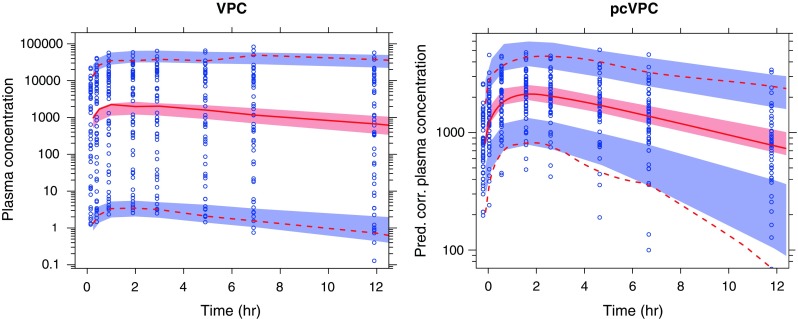
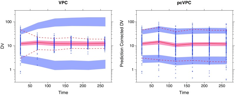
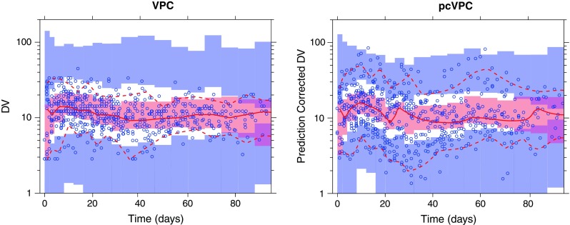
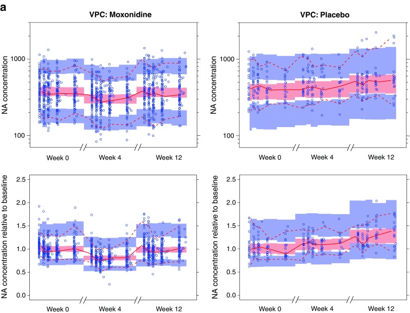
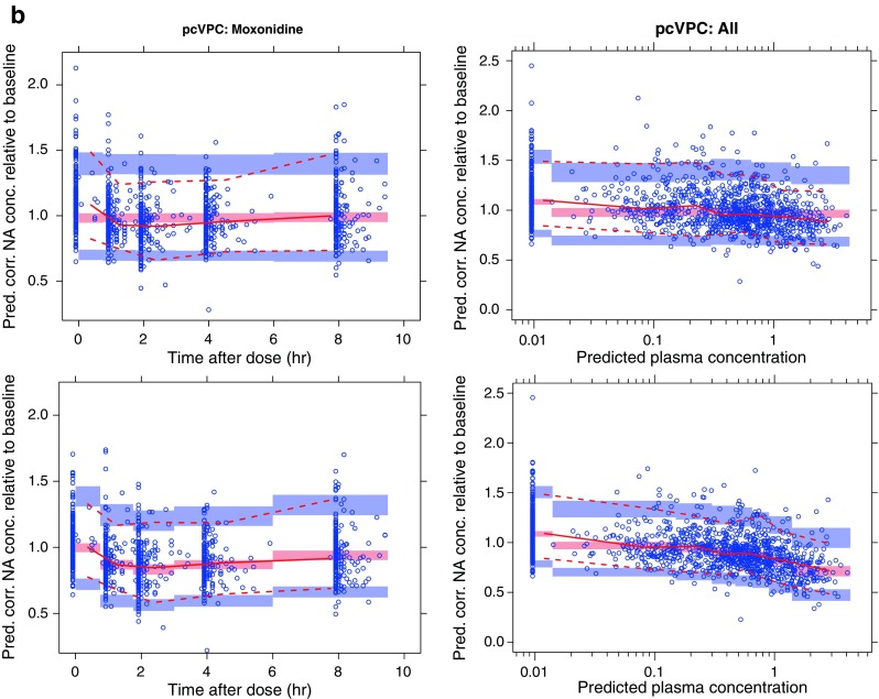
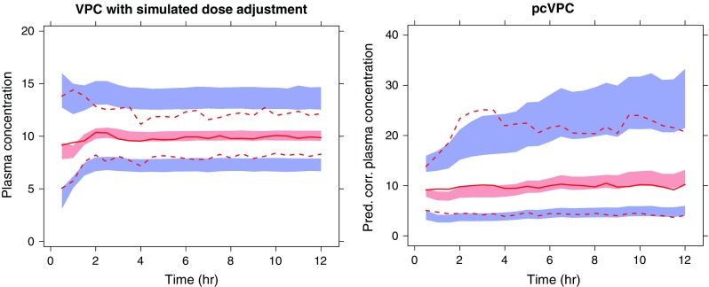
Informative diagnostic tools are vital to the development of useful mixed-effects models. The Visual Predictive Check (VPC) is a popular tool for evaluating the performance of population PK and PKPD models. Ideally, a VPC will diagnose both the fixed and random effects in a mixed-effects model. In many cases, this can be done by comparing different percentiles of the observed data to percentiles of simulated data, generally grouped together within bins of an independent variable. However, the diagnostic value of a VPC can be hampered by binning across a large variability in dose and/or influential covariates. VPCs can also be misleading if applied to data following adaptive designs such as dose adjustments. The prediction-corrected VPC (pcVPC) offers a solution to these problems while retaining the visual interpretation of the traditional VPC. In a pcVPC, the variability coming from binning across independent variables is removed by normalizing the observed and simulated dependent variable based on the typical population prediction for the median independent variable in the bin. The principal benefit with the pcVPC has been explored by application to both simulated and real examples of PK and PKPD models. The investigated examples demonstrate that pcVPCs have an enhanced ability to diagnose model misspecification especially with respect to random effects models in a range of situations. The pcVPC was in contrast to traditional VPCs shown to be readily applicable to data from studies with a priori and/or a posteriori dose adaptations.

Fig. 1

A simulated example of a SAD study with a 10,000-fold dose range and nonlinear pharmacokinetics. The diagnosed model lacked any form of estimated correlation between Vmax and volume of distribution (neither a common covariate nor estimated BSV correlation). The solid red line represents the median observed plasma concentration (nanogram per liter; prediction-corrected plasma concentration in the pcVPC to the right), and the semitransparent red field represents a simulation-based 95% confidence interval for the median. The observed 5% and 95% percentiles are presented with dashed red lines, and the 95% confidence intervals for the corresponding model predicted percentiles are shown as semitransparent blue fields. The observed plasma concentrations (prediction corrected in the pcVPC) are represented by blue circles

Fig. 2

Example with a posteriori dose adaptation (TDM) based on observed trough plasma concentration (units per liter) monitoring over time. Traditional VPC (left) and pcVPC (right), with 95% interpercentile range, for the true model applied to a simulated dataset. Graphical interpretation as in Fig. 1

Fig. 3

Simulation-based diagnostic plots for tacrolimus plasma concentration (nanogram per milliliter) versus time (days). Traditional VPC (left) and pcVPC (right), with 90% interpercentile range, for the final published model (8). Graphical interpretation as in Fig. 1

Fig. 4

a VPCs (90% PI) for noradrenaline (NA) concentration (nanogram per liter) following moxonidine (left) or placebo (right) treatment. The plots in the upper row depict noradrenaline concentration (nanogram per liter) versus time, and the lower row depicts noradrenaline concentration over individual baseline estimate versus time. Time is presented on a broken x-axis with between 0 and 10 h after dose for the first dose and doses following 4 and 12 weeks of moxonidine treatment. Simulations are performed with a nonfinal model with nonconcentration-dependent treatment effect on disease progression. b pcVPCs (90% PI) for NA concentration (nanogram per liter) relative to individual baseline estimate. pcVPCs in the two upper plots are generated using the same nonfinal model that was used for the VPCs in Fig. 4a. The two bottom row pcVPCs are generated with a model including also a concentration-dependent symptomatic effect of moxonidine

Fig. 4

a VPCs (90% PI) for noradrenaline (NA) concentration (nanogram per liter) following moxonidine (left) or placebo (right) treatment. The plots in the upper row depict noradrenaline concentration (nanogram per liter) versus time, and the lower row depicts noradrenaline concentration over individual baseline estimate versus time. Time is presented on a broken x-axis with between 0 and 10 h after dose for the first dose and doses following 4 and 12 weeks of moxonidine treatment. Simulations are performed with a nonfinal model with nonconcentration-dependent treatment effect on disease progression. b pcVPCs (90% PI) for NA concentration (nanogram per liter) relative to individual baseline estimate. pcVPCs in the two upper plots are generated using the same nonfinal model that was used for the VPCs in Fig. 4a. The two bottom row pcVPCs are generated with a model including also a concentration-dependent symptomatic effect of moxonidine

Fig. 5

A simulated example where a loading dose was given followed by a constant infusion. The infusion rate was altered to achieve the target concentration of 10 units. The true underlying model is a one-compartment model with autoinduction of CL. A simple one-compartment model without autoinduction has been fitted to the data. The left hand VPC has been simulated using the same dose alteration algorithm as in the original study. The pcVPC (right) have been simulated using only the realized design. Outer percentiles (dashed red lines) are 2.5% and 97.5% (95% interpercentile range), the semitransparent blue fields are the corresponding model-based confidence intervals, the solid red line represents the observed median, and the semitransparent red field represents the corresponding model-based confidence interval. The actual observations are not plotted in this picture

References

1. Orloff J, Douglas F, Pinheiro J, Levinson S, Branson M, Chaturvedi P, et al. The future of drug development: advancing clinical trial design. Nat Rev Drug Discov. 2009;8(12):949–957. - PubMed
1. Karlsson MO, Savic RM. Diagnosing model diagnostics. Clin Pharmacol Ther. 2007;82(1):17–20. doi: 10.1038/sj.clpt.6100241. - DOI - PubMed
1. Sheiner LB, Beal SL, Dunne A. Analysis of nonrandomly censored ordered categorical longitudinal data from analgesic trials. J Am Stat Assoc. 1997;92(440):1235–1244. doi: 10.2307/2965391. - DOI
1. Holford N. The visual predictive check—superiority to standard diagnostic (Rorschach) plots. PAGE 14 (2005) Abstr 738 [www.page-meeting.org/?abstract=738].
1. Karlsson MO, Holford N. A tutorial on visual predictive checks. PAGE 17 (2008) Abstr 1434 [www.page-meeting.org/?abstract=1434].
Substances
LinkOut - more resources