A reservoir of time constants for memory traces in cortical neurons

Abstract

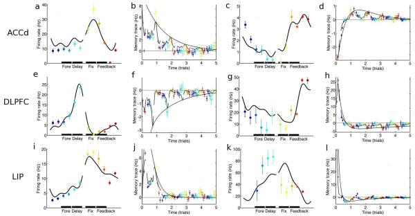
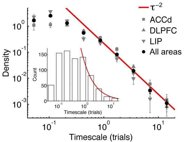
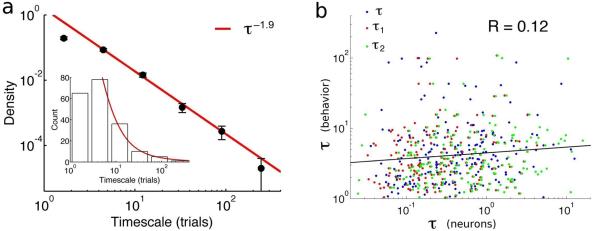
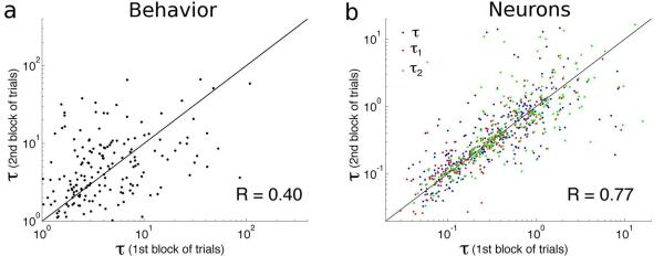
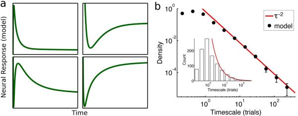
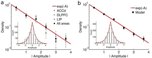
According to reinforcement learning theory of decision making, reward expectation is computed by integrating past rewards with a fixed timescale. In contrast, we found that a wide range of time constants is available across cortical neurons recorded from monkeys performing a competitive game task. By recognizing that reward modulates neural activity multiplicatively, we found that one or two time constants of reward memory can be extracted for each neuron in prefrontal, cingulate and parietal cortex. These timescales ranged from hundreds of milliseconds to tens of seconds, according to a power law distribution, which is consistent across areas and reproduced by a 'reservoir' neural network model. These neuronal memory timescales were weakly, but significantly, correlated with those of monkey's decisions. Our findings suggest a flexible memory system in which neural subpopulations with distinct sets of long or short memory timescales may be selectively deployed according to the task demands.

Figure 1

Behavioral task and schematic illustration of memory traces. (a) In the matching pennies task, the monkey was required to fixate a central spot during the fore-period (500 ms) and delay period (500 ms) while the two choice targets (green disks) were displayed. Then, the central spot disappeared and the monkey made a saccadic eye movement to one of the two choice targets, and maintained its gaze on the chosen target for 500ms (choice fixation). A red ring appearing around the correct target revealed the computer's choice, and if it matched the animal's choice (as illustrated), reward was delivered 500 ms later. Coloured bars at the bottom show the twelve 250ms intervals (epochs) used to compute the firing rates in the analysis. (b,c) Two hypothetical neurons. The neuron in panel b has a constant average firing rate (black line), while the firing rate of neuron in panel c depends on the trial epoch, repeating in each of the three consecutive trials. Red lines show the change in activity due to the outcome in the first trial (continuous line – reward, dashed line – no reward). The inset shows the memory trace of the reward, given by the difference between the red and black lines. The memory trace of neuron in panel b shows a simple decay, while that of neuron in panel c is multiplicatively modulated by the epoch-dependent activity.

Figure 2

An example neuron in ACCd showing multiplicative modulation of memory traces by the epoch code. The colors in all panels denote trial epochs, following the format of Fig.1a. (a) The epoch code for an example neuron, i.e. the firing rate computed in twelve 250ms epochs within a trial and averaged over all trials (black squares, interpolated by the black line, broken during the saccade). Coloured disks correspond to the slopes fitted in panel c (error bars, ±SE); their correlation with the epoch coded quantifies the multiplicative modulation, and is referred to as the factorization index (FI=0.97 in this example). (b) The memory trace f of past rewards in the same neuron, up to five trials in the past. Coloured dots and error bars (±SE) show the results of the multiple linear regression model, Eq.(1), and the black line is the exponential fit (Eq.(2), continuous line, exponential ex(t); broken line, modulated envelope g·ex(t)). The parameters for the fit are shown (A, amplitude; τ, timescale). (c) The memory trace f (from panel b), plotted as a function of the exponential function ex. The lines are least squares fit, each line encompassing a particular epoch and all five trial lags. According to the factorization, the slopes should correspond to the epoch code, f = g·ex. The values of the slopes are plotted in panel a (coloured squares) and compared with the epoch code g(k).

Figure 3

Firing rates and memory traces for six neurons, two for each of the three recorded areas. For each of the six neurons, epoch codes (first and third column) and memory traces (second and fourth column) are shown, in the same format as in Figure 2a and 2b. The second column shows monotonic decay of the memory trace, while the fourth column shows biphasic memory traces (double exponential). Different neurons have different firing rates, both in magnitude and time course, and different types of memory decay, but they are all consistent with an exponential (single or double) decay of the memory modulated by the epoch code. FI's for those neurons are: (a,b) 0.98, (c,d) 0.91, (e,f) 0.98, (g,h) 0.84, (i,j) 0.97, (k,l) 0.61.

Figure 4

Distribution of the timescales characterizing the reward memory traces across neurons. Black disks show the density for the neurons in all three cortical areas in the corresponding bin, i.e. the count of timescales divided by the bin length (error bars: ±SE). The inset shows the count of the timescales in the same bins, in a linear scale (a total of 805 timescales). Grey markers show the density separately for each of the three different cortical areas (square - ACCd, 197 timescales; upward triangle - DLPFC, 362; downward triangle - LIP, 246). The red line (red curve in the inset) shows a power law fit (exponent = −2).

Figure 5

Distribution of behavioral timescales and their relationship with the neural memory timescales. (a) Time constant τ estimated from the learning rate α (τ ~ 1/α) of a reinforcement learning model fit to the monkey's behavioural data. Black disks show the density in the corresponding bin, i.e. the count of timescales divided by the bin length (error bars, ±SE). The inset shows the count of the timescales in the same bins, in linear scale (a total of 196 timescales). The red line (red curve in the inset) shows a power law fit (exponent = −1.9). (b) The scatterplot of behavioural vs neural memory timescales obtained from all sessions where both were available. Neural timescales from different types of fit (τ from single exponential and τ₁, τ₂ from double exponential) are shown in different colours. Behavioral and neural timescales show a small but significant correlation (R=0.12, p=0.003).

Figure 6

Stability of behavioural (a) and neural memory timescales (b) within an experimental session. In both panels, the scatterplot of the timescales fitted in the second half of the trials is plotted against the timescales fitted in the first half of the trials in the same session. The correlation is significantly different from zero in both cases (R=0.4 for behavioural timescales, R=0.77 for neural timescales), suggesting that both types of timescales are fairly stable within a single session. Neural memory timescales from different types of fit (τ from single exponential and τ₁, τ₂ from double exponential) are shown in different colours.

Figure 7

Neural responses (memory traces) in the model and distribution of timescales of the memory traces in model neurons. (a) The memory traces of four model neurons. (b) Black disks show the density of timescales in the corresponding bin, i.e. the count of timescales divided by the bin length (error bars, ±SE). The inset shows the count of the timescales in the same bins, in linear scales (a total of 1000 timescales). The red line (red curve in the inset) shows a power law fit (exponent = −2).

Figure 8

Distribution of amplitudes of the memory traces in the neural data (a) and model (b). In both panels, black disks show the density in the corresponding bin, i.e. the count of timescales divided by the bin length (error bars, ±SE). The inset shows the count of the amplitudes in the same bins, in a linear scale (537 amplitudes in the data, 1000 in the model). Amplitudes are plotted as absolute values, since the distribution is approximately symmetric (symmetry is shown in the inset). Grey markers show the density separately for the three different recorded areas (squares: ACCd, 134 amplitudes, upward triangles: DLPFC, 243, downward triangles: LIP, 160). The red line (red curve in the inset) shows an exponential fit (e^−|A|).

References

1. Kable JW, Glimcher PW. The neurobiology of decision: consensus and controversy. Neuron. 2009;63:733–745. - PMC - PubMed
1. Rushworth MF, Behrens TE. Choice, uncertainty and value in prefrontal and cingulate cortex. Nat. Neurosci. 2008;11(4):389–97. - PubMed
1. Wang X-J. Decision making in recurrent neural circuits. Neuron. 2008;60:215–234. - PMC - PubMed
1. Soltani A, Lee D, Wang X-J. Neural mechanism for stochastic behavior during a competitive game. Neural Networks. 2006;19:1075–1090. - PMC - PubMed
1. Sutton RS, Barto AG. Reinforcement Learning, An Introduction. MIT Press; Cambridge, MA: 1998.
Publication types