A random-effects model for group-level analysis of diffuse optical brain imaging

Abstract

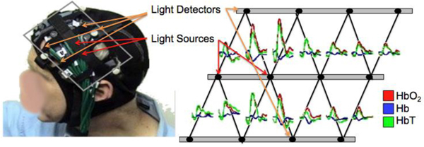
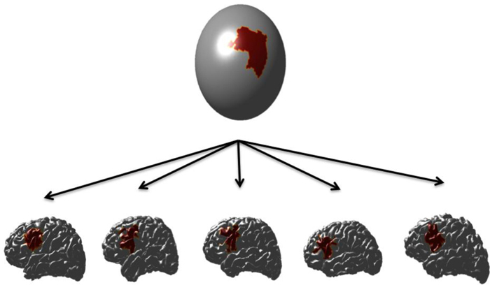
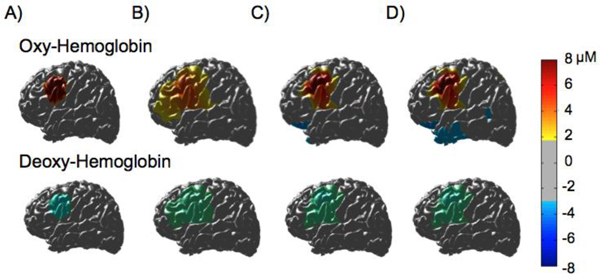
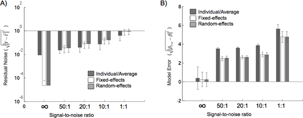
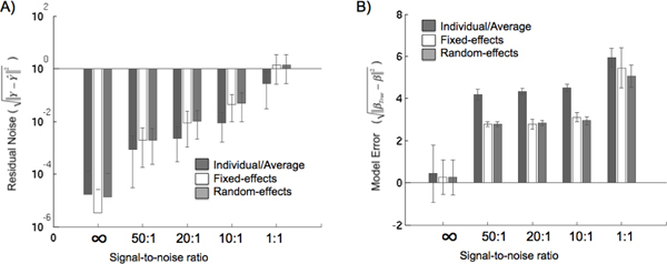
Diffuse optical imaging is a non-invasive technique for measuring changes in blood oxygenation in the brain. This technique is based on the temporally and spatially resolved recording of optical absorption in tissue within the near-infrared range of light. Optical imaging can be used to study functional brain activity similar to functional MRI. However, group level comparisons of brain activity from diffuse optical data are difficult due to registration of optical sensors between subjects. In addition, optical signals are sensitive to inter-subject differences in cranial anatomy and the specific arrangement of optical sensors relative to the underlying functional region. These factors can give rise to partial volume errors and loss of sensitivity and therefore must be accounted for in combining data from multiple subjects. In this work, we describe an image reconstruction approach using a parametric Bayesian model that simultaneously reconstructs group-level images of brain activity in the context of a random-effects analysis. Using this model, we demonstrate that localization accuracy and the statistical effects size of group-level reconstructions can be improved when compared to individualized reconstructions. In this model, we use the Restricted Maximum Likelihood (ReML) method to optimize a Bayesian random-effects model.

Keywords: (170.2655) Functional monitoring and imaging; (170.3010) Image reconstruction techniques.

Fig. 1

Example of optical head cap and evoked response signals. An example of the optical imaging head cap is shown on the left. This cap contains light sources and detectors connected via fiber optics. Each of the nearest-neighbor measurement pairs records changes in the optical absorption of the tissue in between the two positions. During functional studies, the arrangement of sensors can be used to estimate the spatial distribution of oxy- (HbO₂), deoxy- (Hb), and total-hemoglobin (HbT) at each position. The image on the right shows an example data set showing activation in the frontal portion of the probe.

Fig. 2

Schematic of analysis route. The figure above schematically illustrates the steps in the construction of the surface-wavelet model. This model was previously described in [18]. Using a structural MRI, the brain is segmented and then inflated into a spherical representation using the Massachusetts General Hospital’s FreeSurfer tools (www.nmr.mgh.harvard.edu). The cortical surface of the registered brain is used to generate a set of two-dimensional wavelets that depict textures (e.g. brain activity images) on the surface. The segmented brain is also used to construct the optical forward model.

Fig. 3

Multiple resolution surface meshes for head and brain. In this work, a two-layered nested model was used to depict signals originating in the brain and the scalp. Both layers were modeled using a spherical wavelet basis, which is constructed from repeated subdivision of an icosohedral mesh as described in [18]. In panel A, we show the mesh generated for the surface of the brain. The first column shows the mesh at four levels (3-6) of the model and the second column shows the blurring of a 2cm object on the surface of the brain. Panel B shows the mesh (levels 1-4) and smoothing effect of a 2cm object on the surface of the skin.

Fig. 4

Sensitivity of the optical probe. The sensitivity model for the optical probe used in this study (see Fig. 1) is shown panel A. This probe consisted of 4 source and 8 detector positions in a nearest-neighbor arrangement. The relative sensitivity map is shown on the inflated surface of the brain for the Colin27 atlas. The anatomical gyri and sulci locations are indicated in green and blue respectively in panel B. The sensitivity of the optical probe is near zero within the sulci of the brain.

Fig. 5

Skin noise model. In addition to brain activation, a low-spatial frequency noise image was added to the skin layer of the model. This was generated by placing an inclusion with a 5cm radius on the surface of the skin layer followed by spatial smoothing. The skin noise image was randomly placed for each simulation. An example noise image for oxy-hemoglobin is shown above.

Fig. 6

Positions of the optical probe for within subject simulations. Optical data was simulated for displacements of the optical probe of 0.5-15mm. The probe was repositioned five times for each level of displacement error. In panel A, we show the procedure to register the optical probe on the head of a phantom using a Polhemus three-dimensional digitizer. Random perturbations were generated numerically from a registered template. In panel B, the placement of the five probes for the ±15mm displacement simulations is shown. A different color marker represents each position. For simulations, the Colin27 [28] atlas was used.

Fig. 7

Generation of inter-subject simulations. Optical data from multiple subjects was simulated by first generating an activation region on the registered atlas (spherical) map. This activation was then morphed back onto the individual cortical structures for five subjects via FreeSurfer. According to the registration of the cortical surface, the simulated activation in each of the five subjects represents the same anatomical area in the inflated space, however the extent and location in the three-dimensional (folded) brains varies between subjects.

Fig. 8

Intra-subject optical reconstructions from repeated measurements. The images above show the results of a simulation of intra-subject data with a random optical probe displacement of +/−15mm (also see Fig. 6). Data was simulated with a signal-to-noise ratio of 10:1. In column A, the simulated truth images are shown. The top/bottom rows show oxy- and deoxy-hemoglobin respectively. Column B shows the average of five individual reconstructions using a ReML model. Column C and D show the same data reconstructed using a fixed and random-effects model respectively.

Fig. 9

Statistical effects sized from intra-subject optical reconstructions. The images above show the t-statistic for the data presented in Fig. 8. Based on Satterthwaite estimate [24] of the effective degrees-of-freedom for the model (1.8), the cutoff for significance of 0.05 is 3.1 standard deviations. Both the fixed and random effects images (columns C and D respectively) exceed this threshold for the area over the simulated region, but individual reconstruction and averaging results (column B) shows no significant activation.

Fig. 10

Reconstruction errors in within subject simulation. In panel A, the residual error of the model is shown for each of the five signal-to-noise levels and for the individual, fixed, and random-effects model. In panel B, the model error (reconstructed group image minus the simulated image) for the brain is shown.

Fig. 11

Reconstructions of simulated data in inter-subjects study. The images above show the results of a simulation of inter-subject data (N = 5). Data was simulated with a signal-to-noise ratio of 10:1. In column A, the simulated truth images are shown. The top/bottom rows show the reconstructions of oxy-hemoglobin on the registered spherical surface and the group image projected onto one particular cortical surface. Column B shows the average of five individual reconstructions. Column C and D show the same data reconstructed using a fixed and random-effects model respectively.

Fig. 12

Statistical effects of the inter-subjects study. The images above show the t-statistic for the data presented in Fig. 11. As before, the cutoff for significance of p<0.05 is 3.1 standard deviations. Again, both the fixed and random effects images (columns C and D respectively) exceed this threshold for the area over the simulated region, but individual reconstruction and averaging results (column B) shows no significant activation. Column A shows the simulated true image.

Fig. 13

Reconstructed images for the five subjects. Both the individual reconstructions and the random effects model allow recovery of both the group averages (previously shown in Figs. 11 and 12) and the estimates for each individual subject. The individual subjects’ images are recovered from the random-effects model through Eq. (9) and are shown above for the same data presented in Fig. 10. The top row shows the location of the simulated activity on each subject’s brain. Note that the location and extent varies based on the individual folds of the brain. All five activation patterns were generated from the same registered cortically registered brain space (see Fig. 7). The middle row shows the results of the individual reconstructions and the bottom row shows the random-effects model.

Fig. 14

Reconstruction errors in inter-subject simulation. In panel A, the residual error of the model is shown for each of the five signal-to-noise levels and for the individual, fixed, and random-effects model for the data presented in Figs. 11-13. In panel B, the model error (reconstructed group image minus the simulated image) for the brain is shown.

Fig. 15

Image reconstruction of between groups study. The images above show the results of a simulation of two groups of subjects (N = 5/5). The simulated activation in group I and II was 8μm and 4μm respectively for oxy-hemoglobin (column A) and −2μm and −1μm for deoxy-hemoglobin (not shown). Data was simulated with a signal-to-noise ratio of 10:1. Columns B and C show the reconstructions of the two groups using a three and four-level random-effects model respectively. In the three-level model (B), the two groups were reconstructed independently. In the four-level model (C), both groups (10 subjects total) were reconstructed simultaneously.

Fig. 16

Statistical effects of the inter-groups study. The images above show the t-statistic for the data presented in Fig. 15. The cutoff for significance of p<0.05 is 2.2 standard deviations (Satterthwaite correction). For both group's the estimated activation was significant for both the three- and four-level random effects models (columns B and C respectively). The difference image was only significant in the case of the four-level random-effects model (Column C). Column A shows the simulated true image.

References

1. Boas D. A., Dale A. M., Franceschini M. A., “Diffuse optical imaging of brain activation: approaches to optimizing image sensitivity, resolution, and accuracy,” Neuroimage 23(Suppl 1), S275–S288 (2004).10.1016/j.neuroimage.2004.07.011 - DOI - PubMed
1. Okada E., Delpy D. T., “Near-infrared light propagation in an adult head model. II. Effect of superficial tissue thickness on the sensitivity of the near-infrared spectroscopy signal,” Appl. Opt. 42(16), 2915–2922 (2003).10.1364/AO.42.002915 - DOI - PubMed
1. Okada E., Delpy D. T., “Near-infrared light propagation in an adult head model. I. Modeling of low-level scattering in the cerebrospinal fluid layer,” Appl. Opt. 42(16), 2906–2914 (2003).10.1364/AO.42.002906 - DOI - PubMed
1. Kocsis L., Herman P., Eke A., “The modified Beer-Lambert law revisited,” Phys. Med. Biol. 51(5), N91–N98 (2006).10.1088/0031-9155/51/5/N02 - DOI - PubMed
1. Huppert T. J., Allen M. S., Diamond S. G., Boas D. A., “Estimating cerebral oxygen metabolism from fMRI with a dynamic multicompartment Windkessel model,” Hum. Brain Mapp. 30(5), 1548–1567 (2009).10.1002/hbm.20628 - DOI - PMC - PubMed
LinkOut - more resources