An improved coarse-grained model of solvation and the hydrophobic effect

Abstract

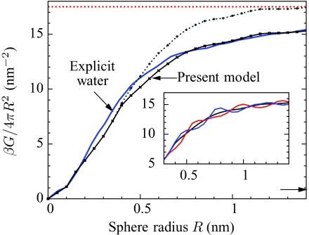
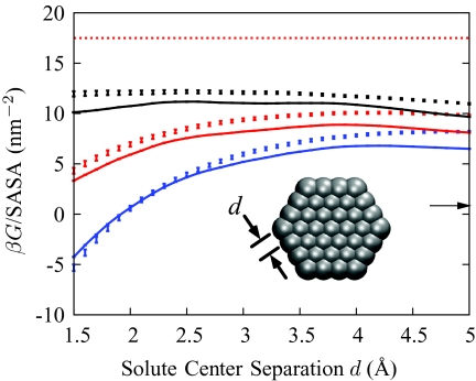
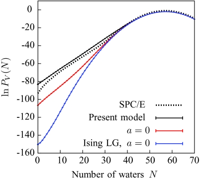
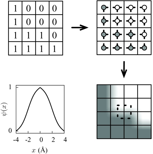
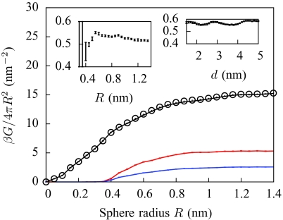
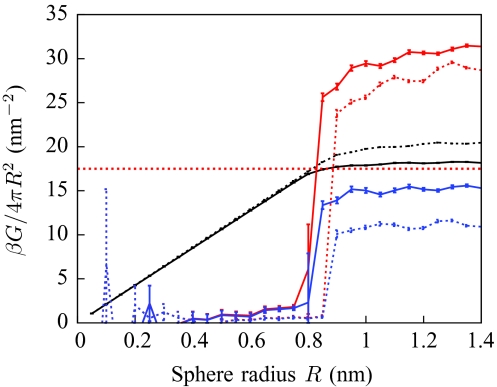
We present a coarse-grained lattice model of solvation thermodynamics and the hydrophobic effect that implements the ideas of Lum-Chandler-Weeks theory [J. Phys. Chem. B 134, 4570 (1999)] and improves upon previous lattice models based on it. Through comparison with molecular simulation, we show that our model captures the length-scale and curvature dependence of solvation free energies with near-quantitative accuracy and 2-3 orders of magnitude less computational effort, and further, correctly describes the large but rare solvent fluctuations that are involved in dewetting, vapor tube formation, and hydrophobic assembly. Our model is intermediate in detail and complexity between implicit-solvent models and explicit-water simulations.

Figure 1

Schematic showing the solute and the large length-scale density field on a grid.

Figure 2

Solvation free energies G of hard spheres of increasing radii, as calculated from explicit SPC∕E water simulations (Ref. 19) (solid blue), from the coarse-grained model (solid black), and from one of the most common variants of GBSA (Ref. 61) (arrow at bottom right). Different parameterizations of GBSA yield nonpolar solvation energies that may differ by as much as a factor of ten, reflecting the crudeness of the SA portion of the model (Ref. 61). When the coarse-grained model has no unbalancing potential (a = 0, dashed gray), the intermediate-size regime is only qualitatively reproduced. For large spheres, the ratio of G to surface area tends to the liquid-vapor surface tension γ (horizontal red dots). Inset: illustration of lattice artifacts. The spheres are centered at different offsets from the lattice: a generic position (0.98, 0.79, 1.89 Å) that breaks all rotational and mirror symmetries (black), a lattice cell corner (blue), and a lattice cell center (red). All three curves are identical for R ⩽ 0.35 nm.

Figure 3

Solvation free energies G of hexagonal plates, as a function of plate size, as calculated by the coarse-grained model (solid lines), by explicit SPC∕E water simulations (points), and by the same GBSA variant as in Fig. 2 (arrow on right). Three values of the attractive interaction strength η are shown: 0.0 (black), 0.5 (red), and 1.0 (blue). Solvent-accessible surface areas (SASAs) were calculated using VMD (Ref. 62) with a particle radius of 1.97 Å, a solvent radius of 1.4 Å, and 1 000 000 samples per atom. The bulk liquid-vapor surface tension of water (horizontal red dots) is shown. Inset: detail of the hexagonal plate. The solvent-excluded volume of each oily site is a sphere of radius R₀ = 3.37 Å.

Figure 4

Water number distribution in a 12 × 12 × 12 ų cube, as obtained using explicit SPC∕E water simulations (Ref. 33), the present model, the present model without the unbalancing potential (a = 0), and a model with an Ising lattice gas and no unbalancing potential.

Figure 5

Water number distributions in a probe volume of size 24 × 24 × 3 Å³ immediately adjacent to a model plate solute (inset) of varying attractive strength η, in the coarse-grained model (solid lines) and in explicit SPC∕E water (points). Defining z = 0 to be the plane passing through the plate center, points in the probe volume (green) satisfy 5 Å < z < 8 Å, so that a water molecule touching the plate is located at the edge of the probe volume (Ref. 33).

Figure 6

Setup for examining water fluctuations under confinement (here, d = 8 Å). The model hydrophobic plates (Ref. 33) (gray particles) are placed d Å apart: taking into account the van der Waals radii of about 2 Å of the plates’ oily particles and the 3 Å thickness of each plate, the center of the first plate is placed at z = 0, the center of the second plate is placed at z = d + 7 Å. The van der Waals radius of water (red and white sticks) being about 1.5 Å, the 24 × 24 × (d − 3) ų probe volume (green) extends from z = 5 Å to z = d + 2 Å. The plates are not perfectly flat, so some waters fit between the plates and the probe volume.

Figure 7

Phase diagram for the interplate region of the system depicted in Fig. 6. For the explicit SPC∕E water simulations (blue), each symbol corresponds to an individual P_V(N) distribution that we have calculated (filled: wet state stable; open: dry state stable). The phase boundary (blue dashes) is estimated from a linear interpolation of the relative stability of the wet and dry states. The relative stability is determined from the relative depths of the basins in −ln P_V(N). The phase boundary for the present model (red solid line) was estimated from a dense sampling of P_V(N) distributions, and is accurate to ±0.1 Å in d and ±0.1 in η.

Figure 8

Water density distribution of confined water 1 Å from coexistence. These distributions are for the system depicted in Fig. 6 when η = 0.5. Coexistence lines are shown in Fig. 7. The explicit water simulation data (black) correspond to d = 11 Å, while the coarse-grained model (red) results correspond to d = 9 Å. The remaining P_V(N) distributions are included in the Supplementary Data (Ref. 72).

Figure 9

Constructing n(r) from {n_i}. The binary field specifies whether the density at the center of each lattice cell should be that of the liquid or that of the vapor. Between cell centers, the density is interpolated using the basis function ψ(x) (whose form for water is shown in the lower left panel). The dashed lines delineate the domain of integration of the local free energy h_i given by Eq. 10.

Figure 10

Solvation free energies G of hard spheres as a function of sphere radius, where the term H₊[{n_i}] (Eq. D1) has been included and the renormalization constant K has been set to 1 (solid black), compared to the simpler model in Eq. 13 (circles). The averages of −〈H_int[{n_i}]〉 (red) and 〈H₊[{n_i}]〉 (blue) are nearly proportional to each other. Left inset: implied renormalization constant K, equal to 〈H_int[{n_i}] + H₊[{n_i}]〉∕〈H_int[{n_i}]〉. Note that both the numerator and denominator take on essentially zero value for R ≲ 0.4 nm. Right inset: implied value of K for hexagonal plate solute (Fig. 3) with η = 1.0. The implied value of K is similar for different η.

Figure 11

Solvation free energies G of spheres in the model of Ref. (black), for cell sizes λ = 2.1 Å (solid) and λ = 2.3 Å (dashes). The use of the Ising Hamiltonian causes the average value of H_large[{n_i}] (red) to significantly exceed the solvation free energy, but also leads to large excess entropies (blue, TS = 〈H〉 − G). At λ = 2.1 Å, but not at λ = 2.3 Å, a fortuitous cancellation leads to correct solvation free energies.

References

1. Kauzmann W., Adv. Protein Chem. 14, 1 (1959).10.1016/S0065-3233(08)60608-7 - DOI - PubMed
1. Tanford C., The Hydrophobic Effect: Formation of Micelles and Biological Membranes (Wiley, New York, 1973).
1. Alberts B., Johnson A., Lewis J., Raff M., Roberts K., and Walter P., Molecular Biology of the Cell, 5th ed. (Garland Science, New York, 2007).
1. Chandler D., Nature (London) 437, 640 (2005).10.1038/nature04162 - DOI - PubMed
1. Chennamsetty N., Voynov V., Kayser V., Helk B., and Trout B. L., Proc. Natl. Acad. Sci. U.S.A. 106, 11937 (2009).10.1073/pnas.0904191106 - DOI - PMC - PubMed
Publication types