

Single molecule fluorescence image patterns linked to dipole orientation and axial position: application to myosin cross-bridges in muscle fibers
- PMID: 21347442
- PMCID: PMC3035662
- DOI: 10.1371/journal.pone.0016772
Single molecule fluorescence image patterns linked to dipole orientation and axial position: application to myosin cross-bridges in muscle fibers
Abstract
Background: Photoactivatable fluorescent probes developed specifically for single molecule detection extend advantages of single molecule imaging to high probe density regions of cells and tissues. They perform in the native biomolecule environment and have been used to detect both probe position and orientation.
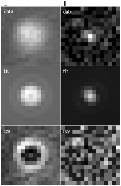
Methods and findings: Fluorescence emission from a single photoactivated probe captured in an oil immersion, high numerical aperture objective, produces a spatial pattern on the detector that is a linear combination of 6 independent and distinct spatial basis patterns with weighting coefficients specifying emission dipole orientation. Basis patterns are tabulated for single photoactivated probes labeling myosin cross-bridges in a permeabilized muscle fiber undergoing total internal reflection illumination. Emitter proximity to the glass/aqueous interface at the coverslip implies the dipole near-field and dipole power normalization are significant affecters of the basis patterns. Other characteristics of the basis patterns are contributed by field polarization rotation with transmission through the microscope optics and refraction by the filter set. Pattern recognition utilized the generalized linear model, maximum likelihood fitting, for Poisson distributed uncertainties. This fitting method is more appropriate for treating low signal level photon counting data than χ(2) minimization.
Conclusions: Results indicate that emission dipole orientation is measurable from the intensity image except for the ambiguity under dipole inversion. The advantage over an alternative method comparing two measured polarized emission intensities using an analyzing polarizer is that information in the intensity spatial distribution provides more constraints on fitted parameters and a single image provides all the information needed. Axial distance dependence in the emission pattern is also exploited to measure relative probe position near focus. Single molecule images from axial scanning fitted simultaneously boost orientation and axial resolution in simulation.
Conflict of interest statement
Figures
 ,
,  and
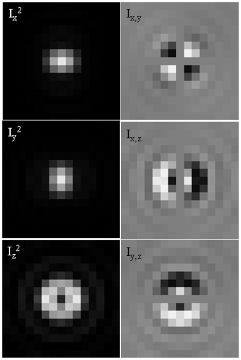
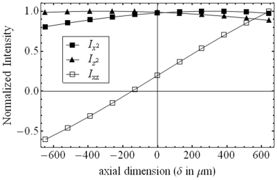
and  from eqs. 14 & 15 show peaks for
  and
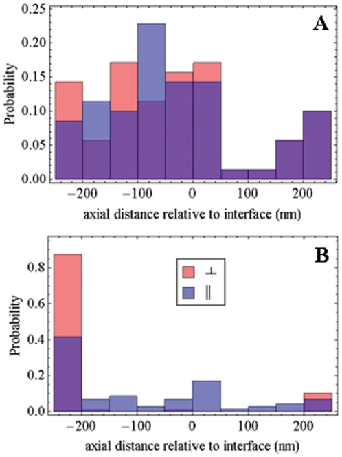
and  occur at different axial positions.
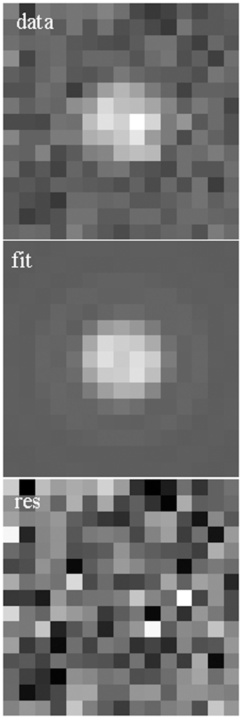
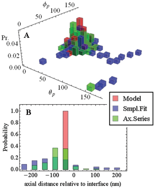
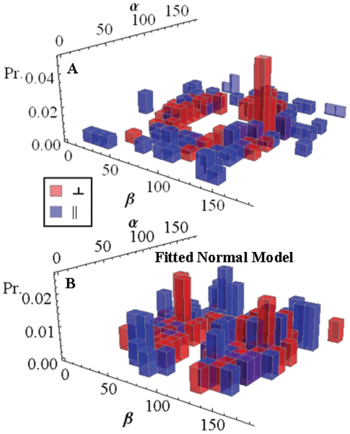
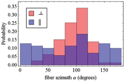
 in fiber-coordinates (α,β) for perpendicular polarized photoactivation (red) and parallel polarized photoactivation (blue) detected from PA-GFP tagged muscle fibers in rigor. Panel B: The orientation distribution for
  in fiber-coordinates derived from simulated data from the model distribution in eq. 17 for β0 = 47, σβ = 20, γB,0 = 0, and σγ = 1 degrees. Simulated data was fitted by the pattern recognition method used to fit the muscle fiber data shown in Panel A.
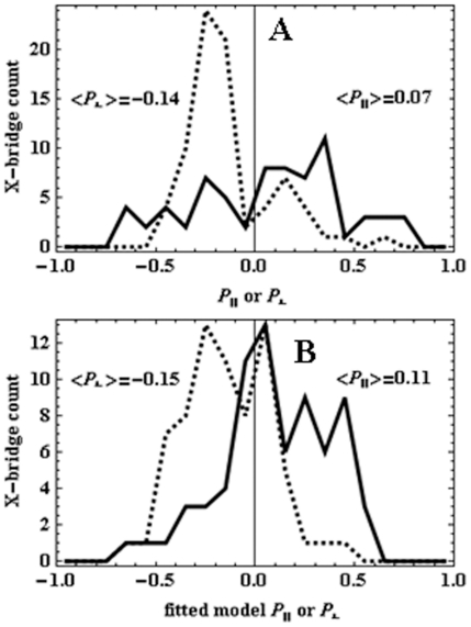
Similar articles
-
GFP-tagged regulatory light chain monitors single myosin lever-arm orientation in a muscle fiber.Biophys J. 2007 Sep 15;93(6):2226-39. doi: 10.1529/biophysj.107.107433. Epub 2007 May 18. Biophys J. 2007. PMID: 17513376 Free PMC article.
-
In vivo orientation of single myosin lever arms in zebrafish skeletal muscle.Biophys J. 2014 Sep 16;107(6):1403-14. doi: 10.1016/j.bpj.2014.07.055. Biophys J. 2014. PMID: 25229148 Free PMC article.
-
Mapping microscope object polarized emission to the back focal plane pattern.J Biomed Opt. 2009 May-Jun;14(3):034036. doi: 10.1117/1.3155520. J Biomed Opt. 2009. PMID: 19566329 Free PMC article.
-
Measuring rotations of a few cross-bridges in skeletal muscle.Exp Biol Med (Maywood). 2006 Jan;231(1):28-38. doi: 10.1177/153537020623100104. Exp Biol Med (Maywood). 2006. PMID: 16380642 Review.
-
Recent advances in super-resolution fluorescence imaging and its applications in biology.J Genet Genomics. 2013 Dec 20;40(12):583-95. doi: 10.1016/j.jgg.2013.11.003. Epub 2013 Nov 23. J Genet Genomics. 2013. PMID: 24377865 Review.
Cited by
-
Resolving cargo-motor-track interactions with bifocal parallax single-particle tracking.Biophys J. 2021 Apr 20;120(8):1378-1386. doi: 10.1016/j.bpj.2020.11.2278. Epub 2020 Dec 25. Biophys J. 2021. PMID: 33359832 Free PMC article.
-
Optimized measurements of separations and angles between intra-molecular fluorescent markers.Nat Commun. 2015 Oct 16;6:8621. doi: 10.1038/ncomms9621. Nat Commun. 2015. PMID: 26509412 Free PMC article.
-
Auxotonic to isometric contraction transitioning in a beating heart causes myosin step-size to down shift.PLoS One. 2017 Apr 19;12(4):e0174690. doi: 10.1371/journal.pone.0174690. eCollection 2017. PLoS One. 2017. PMID: 28423017 Free PMC article.
-
Evanescent field shapes excitation profile under axial epi-illumination.J Biomed Opt. 2012 Jun;17(6):066021. doi: 10.1117/1.JBO.17.6.066021. J Biomed Opt. 2012. PMID: 22734777 Free PMC article.
-
In vivo myosin step-size from zebrafish skeletal muscle.Open Biol. 2016 May;6(5):160075. doi: 10.1098/rsob.160075. Epub 2016 May 25. Open Biol. 2016. PMID: 27249818 Free PMC article.
References
-
- Bobroff N. Position measurement with a resolution and noise-limited instrument. Rev Sci Instrum. 1986;57:1152–1157.
-
- Betzig E, Chichester RJ. Single molecules observed by near-field scanning optical microscopy. Science. 1993;262:1422–1425. - PubMed
-
- Hellen EH, Axelrod D. Fluorescence emission at dielectric and metal-film interfaces. Journal of the Optical Society of America B. 1987;4:337–350.
Publication types
MeSH terms
Substances
Grants and funding
LinkOut - more resources
Full Text Sources
