Time and Associative Learning

Abstract

In a basic associative learning paradigm, learning is said to have occurred when the conditioned stimulus evokes an anticipatory response. This learning is widely believed to depend on the contiguous presentation of conditioned and unconditioned stimulus. However, what it means to be contiguous has not been rigorously defined. Here we examine the empirical bases for these beliefs and suggest an alternative view based on the hypothesis that learning about the temporal relationships between events determines the speed of emergence, vigor and form of conditioned behavior. This temporal learning occurs very rapidly and prior to the appearance of the anticipatory response. The temporal relations are learned even when no anticipatory response is evoked. The speed with which an anticipatory response emerges is proportional to the informativeness of the predictive cue (CS) regarding the rate of occurrence of the predicted event (US). This analysis gives an account of what we mean by "temporal pairing" and is in accord with the data on speed of acquisition and basic findings in the cue competition literature. In this account, learning depends on perceiving and encoding temporal regularities rather than stimulus contiguities.

Figure 1

Schematic of the experimental protocols by which (Rescorla, 1968) demonstrated that CS-US contingency, not the temporal pairing of the CS and US, produces a US-anticipatory response (CR). The temporal pairing of CS and US is identical in the two groups, but there is no CS-US contingency in the second group (the truly random control), because the US occurs as frequently in the absence of the CS as in its presence, that is, λ_CS = λ_C. The subjects in the Group 1 develop a conditioned response to the CS; the subjects in Group 2 do not. (They did, however, develop a conditioned response to the context, that is, to the experimental chamber.) This was one of the findings that called into question the foundational assumption that the learning mechanism was activated by the temporal pairing of CS and US. CS=the conditioned stimulus (e.g., a tone); US = the unconditioned stimulus (e.g., shock to the feet); ITI=intertrial interval; T=duration of a CS presentation.

Figure 2

Acquisition speed as a function of the duration of the trial CS. Pigeons were exposed to keylight CSs paired with food, at fixed delays that ranged from 4 s to 32 s. For some groups (red line), the intertrial interval (ITI) was fixed at 48 s. As the delay (T) from CS onset to US presentation increased, the number of pairings before the appearance of the CR increased. For other groups (blue line), the ITI was increased in proportion to T. In these groups, trials to acquisition was constant. (Data from Gibbon et al., 1977.)

Figure 3

The effects of fixing the CS duration and varying the trace interval from the offset of the CS until the US is presented. Rats were exposed to a 6-s tone paired with food, with a 6- or 18-s trace interval. Anticipatory head entries into the feeding hopper were recorded. Left: The longer the trace interval, the less the average response rate during the CS. Right: Rate of responding as a function the CS-US interval. The break in the plots occurs at CS offset. Note the steady, appropriately-timed increase during the gap between CS offset and US onset.

Figure 4

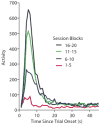
CR timing as training progresses (Drew et al., 2005). Goldfish were exposed to a 5-s visual CS, terminating with an aversive stimulus (US). These training trials were intermixed with probe trials, during which the CS remained on for 45 s, with no US. Movement as a function of time in the CS is shown for blocks of 50 CS-US pairings (5 sessions per block with 10 trials per session). The average amount of anticipatory activity increased as training progressed, but the timing of the CR was appropriate even in the earliest part of training.

Figure 5

Data from a single subject in an eyeblink conditioning experiment reported by Ohyama & Mauk (2001). A: Subject first received CS-US pairings with a 700 ms CS-US interval. The blue part of the tracing shows the period in which the CS was presented. Note the absence of conditioned (anticipatory) blinks during this interval (the rise, that is blink onset, occurs after the blue when the US is presented). Training was stopped before subjects made anticipatory CRs. B: After the trials shown in A, the CS-US interval was reduced to 250 ms and training continued until the subject reliably blinked in anticipation of the US, as shown by these traces in which blink onset occurs during the CS (in blue). C: Traces from probe trials in which the CS remained on for 1250 ms. Subject often blinked twice, with the second blink occurring at around 700 ms. Subjects trained with only one CS-US interval did not show these double blinks.

Figure 6

The integration of temporal information derived from separated experiences. During the first phase of the experiments all groups received 8 pairings of a white noise and a clicker. In the Forward Group the noise preceded the clicker and in the Backward Group the noise followed the clicker. In the second phase all subjects received backward pairing of the food followed by the clicker. Traditional associative theories predict that the clicker will be weakly associated with food because of the backward pairings. Consistent with this view subjects responded very little when tested on the clicker. Consequently, traditional theories predict little responding to the noise. In contrast, the bottom rows on the left side of the figure shows the predictions based on the hypothesis that the temporal information is integrated across the two experiences. As the line above the test CS indicates, subjects in the Forward Group should come to expect the food near the termination of the white noise and show greater anticipation of food whereas subjects in the Backward Group have no basis for expecting food during the noise cue. The right panel shows that this was indeed the case subjects in the Forward Group responded at a significantly higher rate than subjects in the Backward Group when tested with the noise CS.

Figure 7

Relations among information flow, uncertainty, and the US rate. The red curve is the plot of Equaton (1), information flow (bits per second) from a random rate process as a function of the rate. The green curve is the plot of Equation (2), uncertainty per event as a function of the rate. As the rate at which events occur goes up, the flow of information (bits per unit time) increases while the uncertainty about when the next event will occur decreases.

Figure 8

The average suppression ratios for the experimental groups in which contingency was manipulated (Rescorla, 1968). The suppression ratios are plotted as a function of the bits of information that the CS conveys about the time of expected US presentation. The regression line, Y= −0.16X + 0.47, accounts for 88% of the variance. The number pairs by each datum give the λ_CS and λ_ITI for the group of subject from with the datum comes (in USs/2 minutes)

Figure 9

Timeline schematic of the Durlach (1983) experiment. Subjects were first trained with the white CS, which unfailingly predicted the food US (dot) at the end of its 10-s duration. Then, subjects were divided into two groups to be trained with the gray CS. For one group (top line), the US was no more frequent when the CS was on than when it was not on, as in Rescorla’s (1968) truly random control experiment. As in Rescorla’s experiment, this group did not develop a CR to the gray CS. The second group (second line) had the same ITI reinforcements (the reinforcements unsignaled by the gray CS), but these reinforcements were signaled by the white CS. This group did develop a conditioned response to the gray CS. The third line shows the effective event stream for the gray CS, when the white CS-US pairings (and the durations they consume) are excised. This represents the hypothesized treatment of the gray CS if its event stream is segregated from that of the white CS. Now the contingency between the gray CS and the remaining dots is obvious (the gray CS provides information about the temporal location of the reinforcements that are “unexplained” by the white CS). Note that the rate of CS reinforcement in the top line (random control group) is the same as the background rate of reinforcement in the absence of the CS. Thus, the expected time to the next reinforcement is independent of whether the CS is or is not present, making the CS uninformative. By contrast, in the bottom line, this same rate is considerably greater than the rate of occurrence of otherwise unexplained USs (reinforcements not attributable to the white CS). Thus, the expected time to reinforcement in the presence of this CS is shorter than in its absence, making the gray CS informative. Because information is both additive and limited by the available information, the information about US occurrence carried by the white CS in line 2 reduces the information provided by the simultaneously present background, thereby increasing the information provided by the gray CS, which competes with this same background.

Figure 10

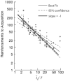
Reinforcements to acquisition as a function of the ratio between the average US-US interval (Ī_C) and the CS-US interval (T) on double-logarithmic coordinates. These speed-of-acquisition data come from a form of Pavlovian conditioning with pigeons called autoshaping, in which the illumination of a small circular light CS is followed by a food US. The slope of the regression is not significantly different from -1. Based on an earlier plot (Gibbon & Balsam, 1981) with data from many different labs.

Figure 11

Reinforcement expectation as a function of the time after an event (CS or US) signaling a fixed interval, t_e, to the next reinforcement. The solid green plot is the inverse of the (objective) expected time to reinforcement, 1/(t_e − t), which is infinite when t = t_e and negative when t > t_e. The solid red plot is the subjective hazard function, g (t, t_e, wt_e)(1 − G(t, t_e, wt_e)), where g and G are the Gaussian PDF and CDF, with expectation t_e and standard deviation wt_e (w is the subject’s Weber fraction for temporal intervals. The dashed green plot is the inverse of the subjective survival function, 1/(t_e(1 − G(t, t_e, wt_e))). Note that the (subjective) conditional hazard function drops to zero at CS onset and rises as the time of reinforcement is approached and exceeded. The other two functions jump up from the unconditional (baseline) expectation to 1/t_e and rise further from there. The baseline expectation is, 1/Ī_C, where Ī_C is the average US-US interval. In the case of fixed-time reinforcements with no CS, t = 0 is the time of occurrence of the most recent US and t_e = Ī_C.

References

1. Arcediano F, Escobar M, Miller RR. Temporal integration and temporal backward associations in human and nonhuman subjects. Learning & Behavior. 2003;31(3):242–256. - PubMed
1. Arcediano F, Miller RR. Some constraints for models of timing: A temporal coding hypothesis perspective. Learning and Motivation. 2002;33(1):105–123.
1. Babb SJ, Crystal JD. Discrimination of what, when, and where is not based on time of day. Learning & Behavior. 2006;34(2):124–130. - PubMed
1. Balci F, Gallistel CR, Allen BD, Frank KM, Gibson JM, Brunner D. Acquisition of peak responding: what is learned? Behavioural Processes. 2009;80(1):67–75. - PMC - PubMed
1. Balsam PD. The functions of context in learning and performance. In: Balsam P, Tomie A, editors. Context and Learning. Hillsdale, N.J: Lawrence Erlbaum Associates; 1985.
LinkOut - more resources