Maximum imaging depth of two-photon autofluorescence microscopy in epithelial tissues

Abstract

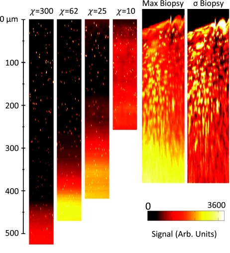
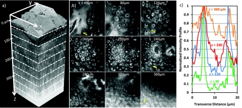
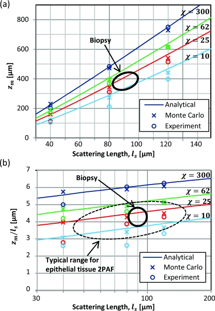
Endogenous fluorescence provides morphological, spectral, and lifetime contrast that can indicate disease states in tissues. Previous studies have demonstrated that two-photon autofluorescence microscopy (2PAM) can be used for noninvasive, three-dimensional imaging of epithelial tissues down to approximately 150 μm beneath the skin surface. We report ex-vivo 2PAM images of epithelial tissue from a human tongue biopsy down to 370 μm below the surface. At greater than 320 μm deep, the fluorescence generated outside the focal volume degrades the image contrast to below one. We demonstrate that these imaging depths can be reached with 160 mW of laser power (2-nJ per pulse) from a conventional 80-MHz repetition rate ultrafast laser oscillator. To better understand the maximum imaging depths that we can achieve in epithelial tissues, we studied image contrast as a function of depth in tissue phantoms with a range of relevant optical properties. The phantom data agree well with the estimated contrast decays from time-resolved Monte Carlo simulations and show maximum imaging depths similar to that found in human biopsy results. This work demonstrates that the low staining inhomogeneity (∼ 20) and large scattering coefficient (∼ 10 mm(-1)) associated with conventional 2PAM limit the maximum imaging depth to 3 to 5 mean free scattering lengths deep in epithelial tissue.

Figure 1

Diagram of the parameters used in quantifying the contrast in 2PAM. The signal and background volumes (V_s and V_b, respectively) and signal and background fluorophore concentrations (C_s and C_b, respectively) are indicated. MS is defined as the fluorescence detected when the geometric focal point of the excitation light is at the center of V_s. MB is defined as the fluorescence detected when the excitation is focused at the same imaging depth as MS, but outside of the feature of interest.

Figure 2

A representative lateral, r, and axial, z, ISPF² from a 100-nm fluorescent bead (a), indicating average lateral and axial FWHMs of 460 and 1760 nm, respectively. The inset shows the two-photon image of a typical bead in the rz-plane. Autocorrelation measurements with a 1 in. singlet lens (b) and with a 20x∕0.95 objective lens (c) indicated duration FWHMs of 185 ± 10 and 270 ± 10 fs, respectively. Double-headed arrows in each plot indicate where the FWHM was measured. Fluorescent signal (Fl) is normalized to 1 at the center of the bead in (a), and at 1.5 ps in (b) and (c).

Figure 3

(a) Schematic of parameters used in modeling signal and background fluorescence generation for a focused Gaussian beam in turbid media. (b) The ratio of signal fluorescence to background fluorescence in a homogeneously stained, R, is a function of the signal volume size, defined here as the volume of a sphere with radius r_s. The lines shown are exact analytical solutions and solid points are Monte Carlo results for focusing to a spot size equal to the measured ISPF² of our system (blue line), and for focusing to the conditions used in our model (red line) in the limiting case where the scattering and absorption of the media are zero.

Figure 4

Monte Carlo simulations are used to calculate the expected fluorescence distribution for an imaging depth of 400 μm in a sample with a 460-nm FWHM lateral spot size, τ_p = 270 fs, l_s = 80 μm, and g = 0.85. These parameters resulted in an R value of 1∕30. (a) shows the lateral and axial distribution of the circumferentially integrated background fluorescence distribution. In this case, most of the background fluorescence comes from above the imaging plane and within 200 μm of the optical axis. (b) shows the contributions from ballistic (B²), scattered (S²), and combined 2(B+S) photons separately. The total fluorescence generation per transverse slice is relatively constant through the first three l_s deep. The solid and dotted lines represent simulations with excitation pulse durations of 270 and 135 fs, respectively. (a) is normalized so that the maximum out-of-focus fluorescence is one, (b) is normalized so the maximum fluorescence is one.

Figure 5

Comparison of XZ images of phantoms with constant scattering length of l_s = 80 μm for increasing staining inhomogeneity, χ, and a human tongue biopsy. Phantom cross sections are maximum projections through 15 μm of Y. Biopsy cross-sections shown are a maximum projection “max Biopsy” and a standard deviation projection “σ Biopsy” through 15 μm of Y. The standard deviation projection is normalized so that the maximum value is white.

Figure 6

Measured sizes of 1 μm diameter fluorescent beads versus depth for l_s = 80 μm, χ = 300 phantom in the lateral and axial directions. The trend and error bars are calculated by the mean and standard deviations of sizes obtained by binning the beads at 50-μm depth increments. We observed no significant increase in bead size and, thus, in system resolution with increasing imaging depth in any of our phantoms.

Figure 7

Plots of normalized fluorescence decays versus imaging depth for constant staining inhomogeneity (χ = 62). Points are data from phantom measurements and lines are the decays predicted by our Monte Carlo simulation with homogeneous (solid lines) and heterogeneous (dashed lines) collection efficiency. (a) The average fluorescence decay, 〈M〉, represents the average pixel value of a 512×512 pixel image recorded at each imaging depth. For comparison, the average fluorescence decay of the biopsy is also shown. (b) Examining relative decays for the MS, MB, and difference (MS-MB) versus depth for the χ = 62, l_s = 80 μm phantom, we found a maximum imaging depth of z_m = 390 μm. (c) The background-subtracted fluorescence decay exhibits exponential decay for the entire measured range. Monte Carlo simulations agree well with experiments for homogeneous collection efficiency (dashed lines) and heterogeneous collection efficiency (solid lines). Decays are normalized to one at 20-μm deep in (a) and (c). In (b), the background is normalized to one at 20-μm deep.

Figure 8

Contrast decays of phantoms with (a) constant staining inhomogeneity and (b) constant scattering length. Monte Carlo simulations (solid lines) agree well with the analytical model (dashed lines) and the phantom contrast measurements (solid dots). Both models slightly overestimate the maximum imaging depth, increasingly at lower staining inhomogeneities.

Figure 9

(a) Three-dimensional rendering of a sequence of 200 lateral 2PAF images acquired from healthy human tongue biopsy. (b) Selection of lateral images from an imaging depth of 40 to 360 μm. Field of view in all lateral images is 170 μm. (c) Normalized signal profile from manually identified cells at imaging depths of 40, 120, 240, and 360 μm. Profiles are taken from lateral lines indicated in (b).

Figure 10

(a) The maximum imaging depth determined by the depth at which Q = 1. (b) Expressing the maximum imaging depth in terms of scattering mean free paths, we observed a linear dependence of maximum imaging depth on log(l_s). Data are plotted from phantom measurements, as well as analytical and Monte Carlo models, with homogeneous collection, and real heterogeneous collection.

References

1. Denk W., Strickler J., and Webb W., “2-Photon laser scanning fluorescence microscopy,” Science 248, 73–76 (1990).10.1126/science.2321027 - DOI - PubMed
1. Masters B. R., So P. T., and Gratton E., “Multiphoton excitation fluorescence microscopy and spectroscopy of in vivo human skin,” Biophys. J. 72, 2405–2412 (1997).10.1016/S0006-3495(97)78886-6 - DOI - PMC - PubMed
1. Koenig K. and Riemann I., “High-resolution multiphoton tomography of human skin with subcellular spatial resolution and picosecond time resolution,” J. Biomedi. Opt. 8, 432–439 (2003).10.1117/1.1577349 - DOI - PubMed
1. Zipfel W. R., Williams R. M., Christie R., Nikitin A. Y., Hyman B. T., and Webb W. W., “Live tissue intrinsic emission microscopy using multiphoton-excited native fluorescence and second harmonic generation,” Proc. Nat. Acad. Sci. U.S.A. 100, 7075–7080 (2003).10.1073/pnas.0832308100 - DOI - PMC - PubMed
1. Skala M. C., Squirrell J. M., Vrotsos K. M., Eickhoff J. C., Gendron-Fitzpatrick A., Eliceiri K. W., and Ramanujam N., “Multiphoton microscopy of endogenous fluorescence differentiates normal, precancerous, and cancerous squamous epithelial tissues,” Cancer Res. 65, 1180–1186 (2005).10.1158/0008-5472.CAN-04-3031 - DOI - PMC - PubMed
Publication types