Spatial effects on species persistence and implications for biodiversity

Abstract

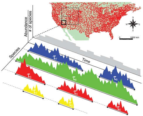
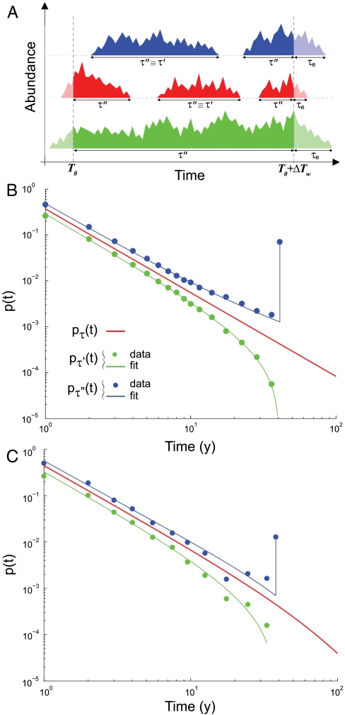
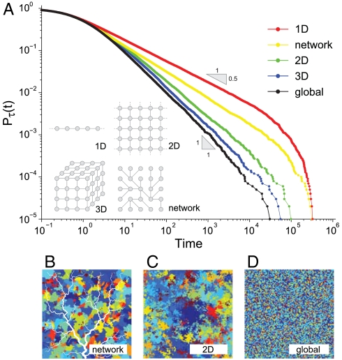
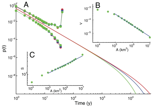
Natural ecosystems are characterized by striking diversity of form and functions and yet exhibit deep symmetries emerging across scales of space, time, and organizational complexity. Species-area relationships and species-abundance distributions are examples of emerging patterns irrespective of the details of the underlying ecosystem functions. Here we present empirical and theoretical evidence for a new macroecological pattern related to the distributions of local species persistence times, defined as the time spans between local colonizations and extinctions in a given geographic region. Empirical distributions pertaining to two different taxa, breeding birds and herbaceous plants, analyzed in a framework that accounts for the finiteness of the observational period exhibit power-law scaling limited by a cutoff determined by the rate of emergence of new species. In spite of the differences between taxa and spatial scales of analysis, the scaling exponents are statistically indistinguishable from each other and significantly different from those predicted by existing models. We theoretically investigate how the scaling features depend on the structure of the spatial interaction network and show that the empirical scaling exponents are reproduced once a two-dimensional isotropic texture is used, regardless of the details of the ecological interactions. The framework developed here also allows to link the cutoff time scale with the spatial scale of analysis, and the persistence-time distribution to the species-area relationship. We conclude that the inherent coherence obtained between spatial and temporal macroecological patterns points at a seemingly general feature of the dynamical evolution of ecosystems.

Fig. 1.

Species persistence times. Persistence time τ within a geographic region is defined as the time incurred between a species’ emergence and its local extinction. Recurrent colonizations of a species define different persistence times. The number of species in the ecosystem as a function of time (gray shaded area) crucially depends on species emergences and persistence times. We analyze two long-term datasets about North America breeding birds (22) and herbaceous plants from Kansas prairies (23). (Inset) Observational routes of the Breeding Bird Survey. Aggregating local information comprised in a given geographic area, we reconstruct species presence–absence time series that allow the estimation of persistence-time distributions.

Fig. 2.

Empirical persistence-time distributions. (A) A schematic representation of the variables that can be measured from empirical data over a time window ΔT_w: τ^′, persistence times that start and end inside the observational window, and τ^′′ , which comprises τ^′ and all the portions of persistence times seen inside the time window that start or/and end outside. Times to local extinction τ_e are also presented. (B) Breeding birds and (C) herbaceous plants probability density function p(t) of τ^′ (green), τ^′′ (blue), and persistence time τ (red). Filled circles and solid lines show observational distributions and fits, respectively. The best fit is achieved with p_τ(t) ∝ t^-α with α = 1.83 ± 0.02 and α = 1.78 ± 0.08 for breeding birds and herbaceous plants, respectively. Note that previous estimates (6) for B are revisited here in the light of the tools developed and of a longer dataset. The spatial scale of analysis is A = 10,000 km² and ΔT_w = 41 y for B and A = 1 m² and ΔT_w = 38 y for C. The finiteness of the time window imposes a cutoff to p_τ^′(t) and an atom of probability in t = ΔT_w to p_τ^′′(t), which corresponds to the fraction of species that are always present during the observational time. p_τ(t) and p_τ^′(t) have been shifted in the log–log plot for clarity.

Fig. 3.

Persistence-time distributions are dependent on the structure of the spatial interaction networks. (A) Persistence-time exceedance probabilities P_τ(t) (probability that species’ persistence times τ be ≥t) for the neutral individual-based model (15, 16) with nearest-neighbor dispersal implemented on the different topologies shown in the inset. Note that in the power-law regime if p_τ(t) scales as t^-α, P_τ(t) ∝ t^-α+1. The scaling exponent α is equal to 1.50 ± 0.01 for the one-dimensional lattice (red), α = 1.62 ± 0.01 for the networked landscape (yellow), 1.82 ± 0.01 and 1.92 ± 0.01, respectively, for the 2D (green) and 3D (blue) lattices. Errors are estimated through the standard bootstrap method. The persistence-time distribution for the mean-field model (global dispersal) reproduces the exact value α = 2 (black curve). For all simulations ν = 10^-5 and time is expressed in generation time units (11). (Bottom) Sketches of the color-coded spatial arrangements of species in a networked landscape (B), in a two-dimensional lattice with nearest-neighbor dispersal (C), and with global dispersal (D).

Fig. 4.

Biogeography of species persistence time. (A) Observational distributions p_τ^′(t) and p_τ^′′(t) (interpolated solid circles) for the breeding bird dataset and corresponding fitted persistence-time distributions p_τ(t) ∝ t^-αe^-νt (solid lines) for different scales of analysis: Area A = 8.5·10⁴ km² (green), A = 3.4·10⁵ km² (blue), A = 9.5·10⁵ km² (red). ν(A) provides the cutoff for the distribution, whose scaling exponent is unaffected by geographic area. Note that the position of the cutoff of p_τ(t) is inferred from the estimate of the atom of probability of p_τ^′′(t), which is more sensitive to the scale of analysis. (B) Scaling of the diversification rate ν with the geographic area ν ∝ A^-β, β = 0.84 ± 0.01. (C) Empirical species-area relationship (SAR). The plot shows the mean number of species S found in moving squares of size A. We find S ∝ A^z, z = 0.31 ± 0.02. Slope and confidence interval have been obtained averaging 41 SARs, one per year of observation.

References

-
- Diamond J. The present, past and future of human-caused exctinctions. Philos Trans R Soc London B. 1989;325:469–477. - PubMed
- Brown JH. Macroecology. Chicago: Univ Chicago Press; 1995.
- Thomas C, et al. Extinction risk from climate change. Nature. 2004;427:145–148. - PubMed
- Svenning J.-C, Condit R. Biodiversity in a warmer world. Science. 2008;322:206–207. - PubMed
Publication types
MeSH terms
Grants and funding
LinkOut - more resources
Full Text Sources