Axonal branching patterns as sources of delay in the mammalian auditory brainstem: a re-examination

Abstract

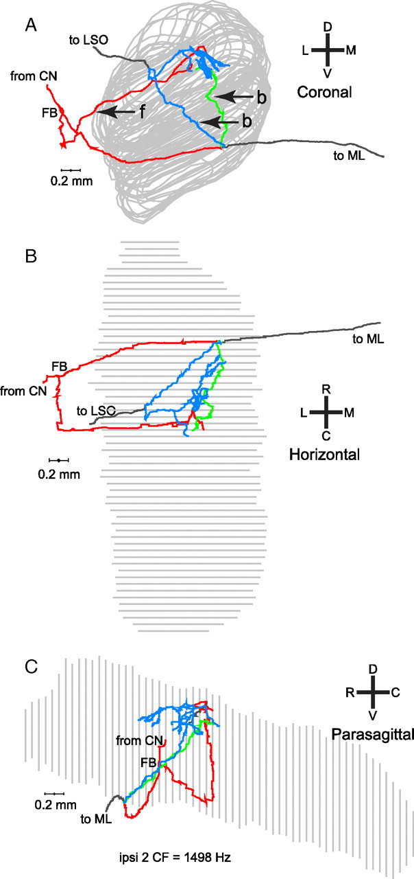
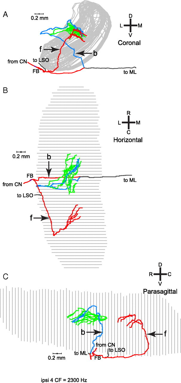
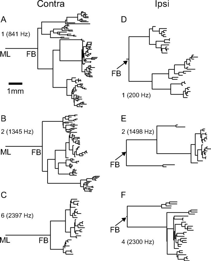
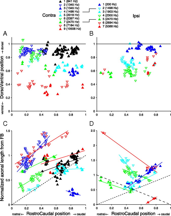
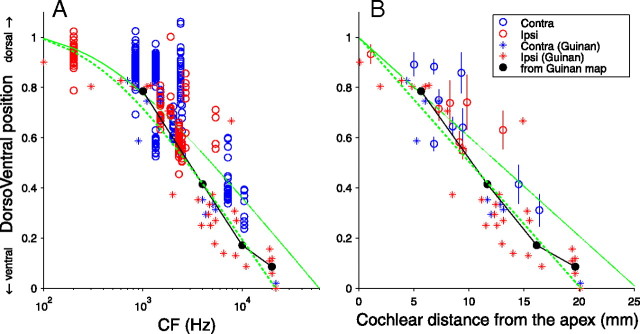
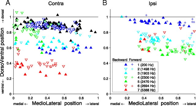
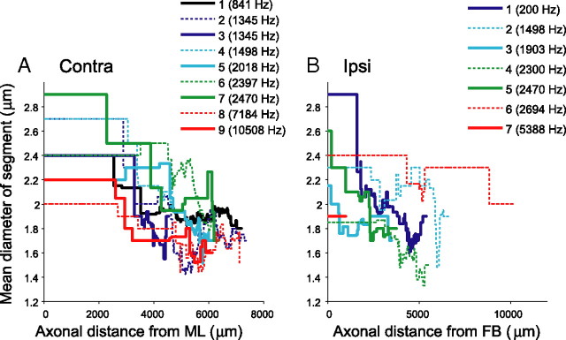
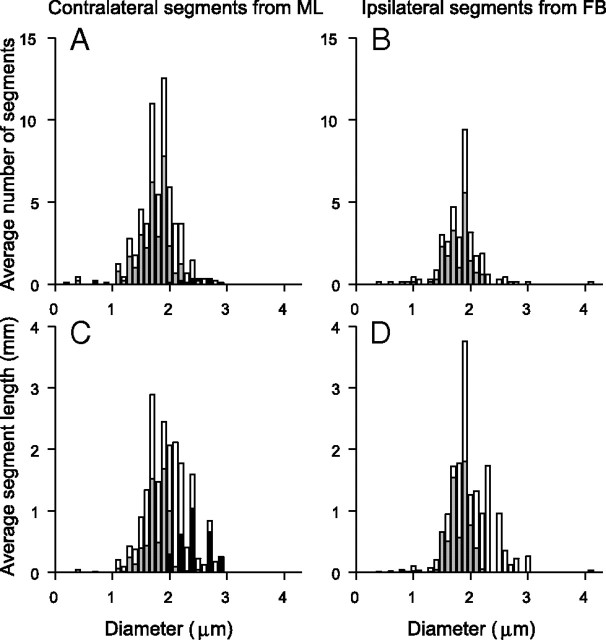
In models of temporal processing, time delays incurred by axonal propagation of action potentials play a prominent role. A pre-eminent model of temporal processing in audition is the binaural model of Jeffress (1948), which has dominated theories regarding our acute sensitivity to interaural time differences (ITDs). In Jeffress' model, a binaural cell is maximally active when the ITD is compensated by an internal delay, which brings the inputs from left and right ears in coincidence, and which would arise from axonal branching patterns of monaural input fibers. By arranging these patterns in systematic and opposite ways for the ipsilateral and contralateral inputs, a range of length differences, and thereby of internal delays, is created so that the ITD is transformed into a spatial activation pattern along the binaural nucleus. We reanalyze single, labeled, and physiologically characterized axons of spherical bushy cells of the cat anteroventral cochlear nucleus, which project to binaural coincidence detectors in the medial superior olive (MSO). The reconstructions largely confirm the observations of two previous reports, but several features are observed that are inconsistent with Jeffress' model. We found that ipsilateral projections can also form a caudally directed delay line pattern, which would counteract delays incurred by caudally directed contralateral projections. Comparisons of estimated axonal delays with binaural physiological data indicate that the suggestive anatomical patterns cannot account for the frequency-dependent distribution of best delays in the cat. Surprisingly, the tonotopic distribution of the afferent endings indicate that low characteristic frequencies are under-represented rather than over-represented in the MSO.

Figure 1.

Illustration of measurements taken within sections. Coronal view of the contralateral projection of a traced fiber (CF, 1345 Hz) superimposed on a Nissl-stained single section, taken at the coronal level of the branch EP, indicated with the yellow dot. Yellow line, Contour of MSO on the section. Yellow asterisks, Most DP and most VP along the long axis of the MSO within the section, which is indicated with black asterisks. Drawing a line through the EP, which is approximately perpendicular to the long axis of the MSO, the arrows show the most medial and lateral points (MB and LB) of the MSO contour on this line. The two other lines (dotted white) indicate the Euclidian distances between EP and VP, and between VP and the DP of this section. Scale bar, 200 μm. Directions are indicated by the cross. D, Dorsal; V, ventral; M, medial; L, lateral.

Figure 2.

Example of the contralateral MSO innervation by one axon (same axon as in Fig. 1). A–C, Coronal (A), horizontal (B), and parasagittal (C) views are shown. The RP and CP were defined as the geometrical center of the most rostral (green line) and most caudal (magenta line) section, respectively. The rostrocaudal position of endpoints was quantified by measuring the Euclidian distance (dashed line) between RP and EP, and was normalized to the distance between RP and CP. The endpoint illustrated is the same one as in Figure 1; the MSO contour outlined in Figure 1 is shown in blue here. ML indicates the point at which the axon crosses the midline. CF of this fiber was 1345 Hz. A computer reconstruction of this fiber was also shown in Smith et al. (1993, their Fig. 4).

Figure 3.

Delay line configuration in 3 contralaterally projecting fibers. A, B, Projections on a parasagittal plane. C, Projection on a horizontal plane. CFs are indicated. Branches that end within the MSO are indicated in red.

Figure 4.

Parasagittal view of 3 more contralateral projections (A–C, with CFs indicated below each reconstruction) with a less clear-cut delay line configuration. In all cases, the FB is located near the center of the rostrocaudal range of EPs. The orientation shown in B applies to all panels. The color convention is as in Figure 3.

Figure 5.

A–C, Coronal (A), horizontal (B), and parasagittal (C) views of a reconstructed projection of one fiber to the ipsilateral MSO. The coronal (A) and horizontal (B) views clearly show the two kinds of ipsilateral branches. One branch originates lateral to the MSO and projects forward (f, red) to it. Two branches originate after the axon has crossed the plane of the MSO and looped back (b, blue and green) to innervate the same region.

Figure 6.

Another example of an ipsilateral MSO projections of one fiber. A, This fiber ran underneath the MSO (coronal view) and also formed forward (f) and backward (b) projecting branches. B, C, The horizontal (B) and parasagittal (C) views reveal that the branches innervate different rostrocaudal portions of the MSO. The backward branches (green and blue) innervated a more rostral portion of the MSO and covered more length of axon from FB than the forward branches.

Figure 7.

A, B, Dendrograms showing the branching pattern and length of axonal segments for three contralateral (A) and three ipsilateral projections (B). The scale bar in A applies to A–F. The horizontal dimension represents the axonal length of branch segments; the vertical dimension is only used to offset these segments and has no meaning with regard to length or order. Fiber number and CF are indicated for each projection. Cross-linking to previous figures with computerized reconstructions is as follows: A = Figure 4A; B = Figures 1 and 2; C = Figure 3A; D = Figure 5 of Smith et al. (1993); E = Figure 5; F = Figure 6.

Figure 8.

Length gradients along the rostrocaudal axis of the MSO. A, B, Distribution of endpoints of contralateral (A) and ipsilateral (B) projections on normalized MSO axes. C, D, Axonal length from FB to the different endpoints. Solid lines are linear regressions. The diagonals with short dashed lines indicate the diagonal of equality; the diagonal with the long dashed lines indicates the slope expected for an opposite length gradient. The caption shows the symbols and color used for the endpoints originating from the different fibers, numbered for increasing CF and reused in subsequent figures. The lines between left and right symbol captions indicate the two fibers for which both the contralateral and ipsilateral projections were reconstructed.

Figure 9.

Tonotopic compression of low frequencies in MSO. A, B, The dorsoventral location, normalized to the dorsoventral extent of the MSO, is shown for all endpoints of all reconstructed fibers on a logarithmic CF abscissa (A) and for their mean and SD on a cochlear distance abscissa (B). Each circle in A indicates a single endpoint (blue, contralateral fiber; red, ipsilateral fiber). The asterisks and the black circles and line show extracellular and summary data from Guinan et al. (1972) (see main text). The green lines are predicted relationships based on the cochlear tonotopic map, based on Greenwood's formula (Greenwood, 1990). The solid green line is the prediction for a full representation of all CFs; the dashed line is for a representation limited to ≤22 kHz. The endpoints at low CFs cluster above the green lines. If low CFs were over-represented in MSO, those endpoints would be expected to cluster below rather than above the green lines.

Figure 10.

A, B, Distribution of endpoints in the coronal plane, for contralateral (A) and ipsilateral (B) projections. Symbol use for A is as in Figure 8. The “Backward” and “Forward” in B refer to backward and forward branches, as illustrated in Figures 5 and 6.

Figure 11.

A, B, Average axon diameters decrease as a function of distance from the midline (A, Contra projections) or from the first branch point (B, Ipsi projections).

Figure 12.

A–D, Distribution of axon diameters does not differ between contralateral (A, C) and ipsilateral (B, D) projections. The top histograms show the average number of segments with a given diameter (0.1 μm bins); the bottom histograms show the corresponding average length (in mm) at that diameter. All histograms are averages calculated for the entire population of contralateral and ipsilateral fibers, normalized to the total number of fibers included. The starting segments were ML (contralateral fibers) and FB (ipsilateral fibers). White bars include all the segments from starting segment to endpoints. Gray bars show length of most distal segments, terminated by endpoints. Black bars show length of most proximal segments, which contain ML (contralateral fibers only).

Figure 13.

Axonal length is linearly related to estimated conduction time. Axonal lengths are measured as in Figures 7 and 11. Conduction time for each endpoint is the sum of conduction times of all segments leading up to that endpoint, calculated from segment length and diameter (see text). Diagrams in A and B illustrate configurations that would result in nonsloping relationships. C, Length and time for contralateral projections, using ML as reference point. D, Length and time for ipsilateral projections, using FB as reference point. One outlying endpoint is clipped off. E, F, Estimated average conduction speeds for all endpoints. This is the slope of the lines connecting the endpoints in C and D with the origin at (0,0), as illustrated with the dashed lines in A and B. E–G, Reference point at (0,0) was ML (E) or FB (F, G). Color code and symbols are identical to Figures 8 and 10. The symbols indicate the lowest and highest speed for the endpoints of a given fiber.

Figure 14.

Rostrocaudal gradients of conduction time. A, B, Relationship between estimated conduction time and location of EP in rostrocaudal dimension in contralateral (A) and ipsilateral (B) fibers. The abscissa is zeroed to the position of the most rostral section in which MSO could be identified, and abscissa values are the distance of endpoints to that most rostral section. Ordinate values are the estimated conduction times from the midline (A, contralateral projections) or first branch point (B, ipsilateral projections). Solid lines are linear regressions. The asterisks at the end of each line indicate the most caudal MSO section. Note that the ordinate in B has a wider range than in A. C, Summary of regression slopes of Figure 8, A and B (abscissa), and of A and B (ordinate). Large symbols indicate values that are significant for both abscissa and ordinate. Contra 4 showed significance (p < 0.05) for length but not for delay; and vice versa for Contra 9. D, Relationship between estimated delay and CF. The anchor point of each colored vertical line at 0 delay represents the RP of the MSO. The opposite end shows the extrapolated delay at the CP (corresponding to the delay accumulated between RP and the asterisk in A and B). The small horizontal bars show the range of delays of the linear regression over which endpoints are present. Symbols and lines at positive delays, in the shaded region, are for fibers with a pattern consistent with the trend observed by Yin and Chan (1990); these are the fibers with positive slope in A or negative slope in B. Symbols and lines at negative delays are for fibers with an opposite branching pattern (negative slope in A or positive slope in B). Hyperbolic curves indicate the π limit (i.e., the extent of one period equaling CF⁻¹). The scale of the abscissa is linear in the left panel and logarithmic in the right panel.

Figure 15.

A, B, Differences in path length between ipsilateral and contralateral inputs. A, Estimated average and range of lengths for contralateral and ipsilateral projections between the FB of the ipsilateral MSO projection and the endpoints. Dashed lines show overall contralateral (C) and ipsilateral (I) mean. B, Schematic of the measurement. The length of the trajectory between midline and contralateral endpoints (red), or between FBi and endpoints (green), was measured (same values as in Fig. 13C,D). To estimate the difference in length of contralateral and ipsilateral inputs, the red segment needs to be augmented by the distance FBi to midline: we use the average measured on ipsilateral projections (4994 μm, see main text). C–F, Absence of length differences in the innervation from the contralateral ear along the dorsoventral dimension of MSO. C, Hypothetical scheme of innervation by contralateral fibers, suggesting extra length for the most dorsally projecting (low-CF) fibers. If input fibers approach the MSO from ventral, low-CF fibers may have longer axonal length (arrow) to innervate the dorsal part of MSO than high-CF fibers for the ventral part. D, relationship between axonal length from ML to endpoints, and CF. Symbols in A and D indicate average axonal length; lines are range (A) and SD (D) for each projection (symbol color and shape as in Fig. 8). E, F, Coronal view of contralateral projections of fibers with lowest and highest CF (840 and 10,508 Hz, respectively).

References

1. Adams JC. Heavy metal intensification of DAB-based HRP reaction product. J Histochem Cytochem. 1981;29:775. - PubMed
1. Beckius GE, Batra R, Oliver DL. Axons from anteroventral cochlear nucleus that terminate in medial superior olive of cat: observations related to delay lines. J Neurosci. 1999;19:3146–3161. - PMC - PubMed
1. Bonham BH, Lewis ER. Localization by interaural time difference (ITD): effects of interaural frequency mismatch. J Acoust Soc Am. 1999;106:281–290. - PubMed
1. Brand A, Behrend O, Marquardt T, McAlpine D, Grothe B. Precise inhibition is essential for microsecond interaural time difference coding. Nature. 2002;417:543–547. - PubMed
1. Brownell WE. Organization of the cat trapezoid body and the discharge characteristics of its fibers. Brain Res. 1975;94:413–433. - PubMed
Publication types
LinkOut - more resources