Comparative Study
. 2011 Feb 23;31(8):3082-94.
doi: 10.1523/JNEUROSCI.4476-10.2011.

A comparison of vestibular spatiotemporal tuning in macaque parietoinsular vestibular cortex, ventral intraparietal area, and medial superior temporal area

Affiliations
Comparative Study

A comparison of vestibular spatiotemporal tuning in macaque parietoinsular vestibular cortex, ventral intraparietal area, and medial superior temporal area

Aihua Chen et al. J Neurosci. .

Abstract

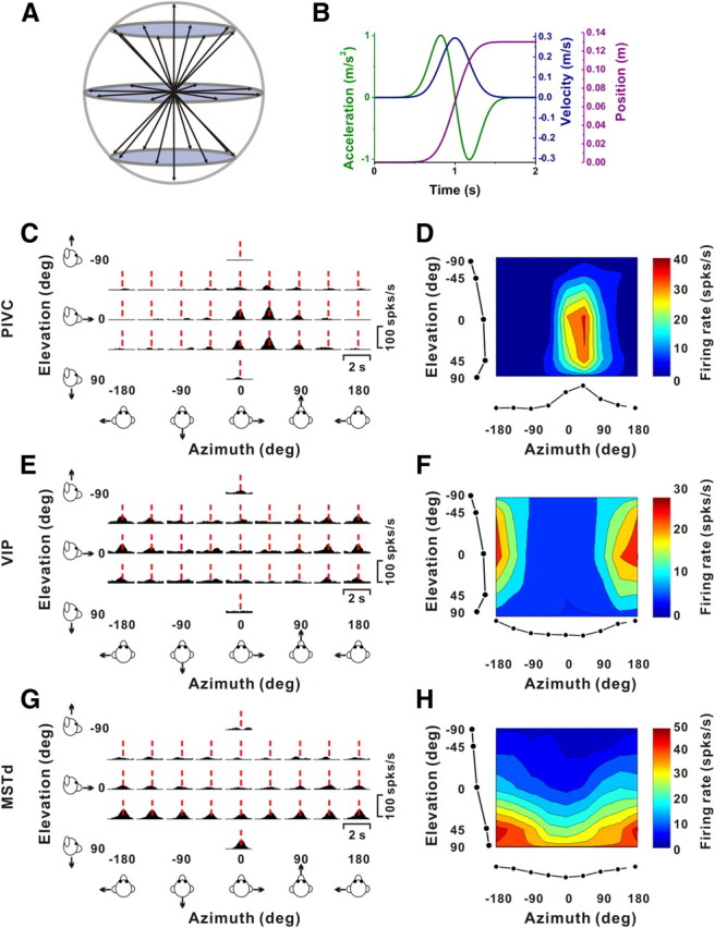
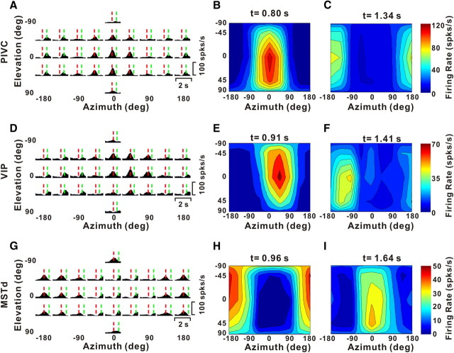
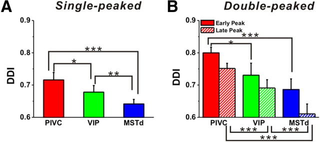
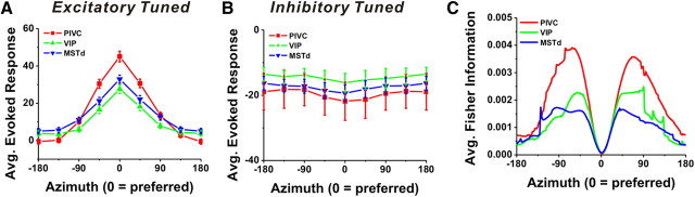
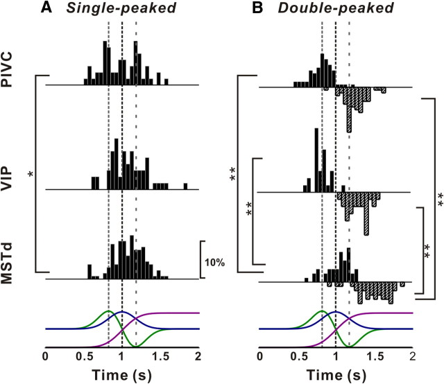
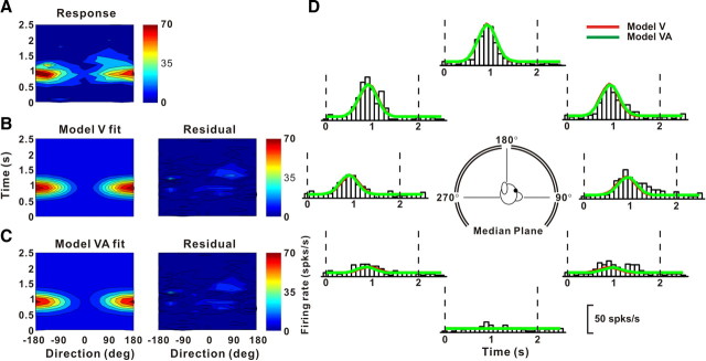
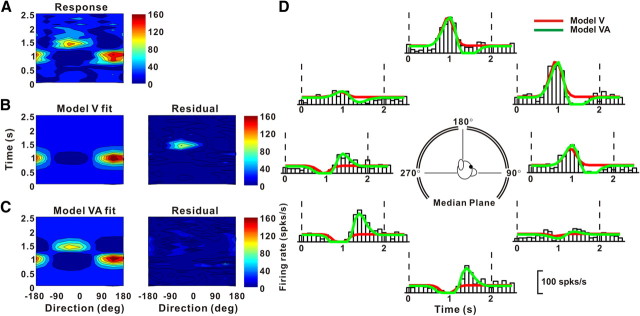
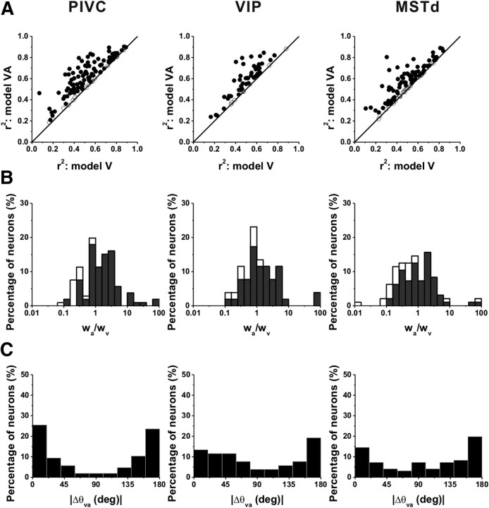
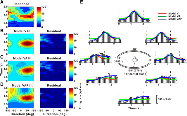
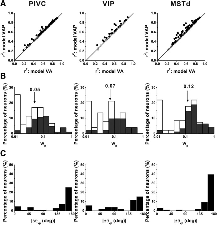
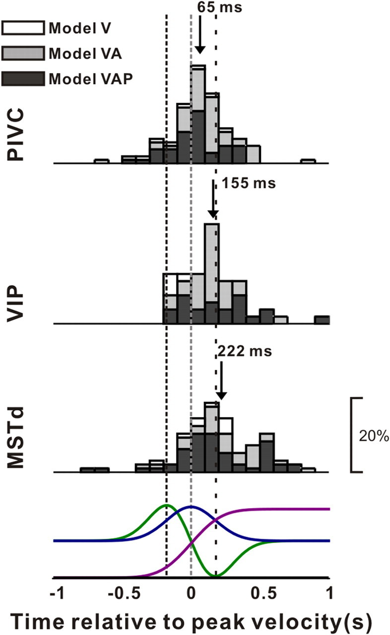
Vestibular responses have been reported in the parietoinsular vestibular cortex (PIVC), the ventral intraparietal area (VIP), and the dorsal medial superior temporal area (MSTd) of macaques. However, differences between areas remain largely unknown, and it is not clear whether there is a hierarchy in cortical vestibular processing. We examine the spatiotemporal characteristics of macaque vestibular responses to translational motion stimuli using both empirical and model-based analyses. Temporal dynamics of direction selectivity were similar across areas, although there was a gradual shift in the time of peak directional tuning, with responses in MSTd typically being delayed by 100-150 ms relative to responses in PIVC (VIP was intermediate). Responses as a function of both stimulus direction and time were fit with a spatiotemporal model consisting of separable spatial and temporal response profiles. Temporal responses were characterized by a Gaussian function of velocity, a weighted sum of velocity and acceleration, or a weighted sum of velocity, acceleration, and position. Velocity and acceleration components contributed most to response dynamics, with a gradual shift from acceleration dominance in PIVC to velocity dominance in MSTd. The position component contributed little to temporal responses overall, but was substantially larger in MSTd than PIVC or VIP. The overall temporal delay in model fits also increased substantially from PIVC to VIP to MSTd. This gradual transformation of temporal responses suggests a hierarchy in cortical vestibular processing, with PIVC being most proximal to the vestibular periphery and MSTd being most distal.


Figures

Figure 1.
Figure 1.
Stimulus parameters and example responses from single-peaked cells. A, Schematic illustration of the 26 3D movement trajectories spaced 45° apart in both azimuth and elevation. B, All movements had a 2 s duration, originated from the center position, and had a Gaussian velocity profile (peak of 30 cm/s, blue) with a corresponding biphasic linear acceleration profile (peak of ±1 m/s2, green) and a sigmoidal displacement of 13 cm (magenta). C, E, G, Response PSTHs for three example neurons from PIVC (C), VIP (E), and MSTd (G). Vertical dashed red lines indicate the respective peak times, when the maximum response across directions occurred. PSTHs were computed with sequential 25 ms bins and then smoothed with a 400 ms sliding window (see Materials and Methods). D, F, H, Corresponding color contour maps showing 3D direction tuning profiles (Lambert cylindrical projection) at peak time (t) for the cells in C (t = 0.94 s, DDI = 0.77), E (t = 0.98 s, DDI = 0.70), and G (t = 1.08 s, DDI = 0.76). Tuning curves along the margins illustrate mean firing rates plotted versus elevation or azimuth (averaged across azimuth or elevation, respectively).
Figure 2.
Figure 2.
Example responses from double-peaked neurons. A, D, G, PSTHs for three example neurons from PIVC (A), VIP (D), and MSTd (G). Vertical dashed red and green lines illustrate the two peak times for each cell. B, C, E, F, H, I, Color contour maps showing 3D direction tuning profiles (Lambert cylindrical projection) at the two peak times (t) for the cells in A (t = 0.80 s, DDI = 0.92 and t = 1.34 s, DDI = 0.86), D (t = 0.91 s, DDI = 0.74 and t = 1.41 s, DDI = 0.70), and G (t = 0.96 s, DDI = 0.74 and t = 1.64 s, DDI = 0.75). The format is as in Figure 1.
Figure 3.
Figure 3.
Population summary of directional tuning strength in areas PIVC (red), VIP (green), and MSTd (blue). A, B, Mean (±SE) values of DDI for single-peaked and double-peaked cells (early peak: solid bars; late peak: hatched bars). Statistical significance (Wilcoxon rank test) of differences is denoted as follows: ***p < 0.001; **0.001 < p < 0.01; *0.01 < p < 0.05.
Figure 4.
Figure 4.
Population summary of directional discrimination in areas PIVC (red), VIP (green), and MSTd (blue). A, Population tuning curves of the excitatory cells in the horizontal plane (PIVC: n = 120, VIP: n = 66, and MSTd: n = 141). B, Population tuning curves of the inhibitory cells in the horizontal plane (PIVC: n = 8, VIP: n = 18, and MSTd: n = 29). Data have been aligned to the peak (for excitatory cells) or trough (for inhibitory cells) response direction of each cell (0°), and spontaneous activity was subtracted before averaging. C, Comparison of averaged Fisher information in the horizontal plane among three areas. Fisher information was aligned to the preferred azimuth direction of each neuron, which is illustrated here as 0°.
Figure 5.
Figure 5.
Distribution of peak times for single-peaked (A) and double-peaked (B) cells in areas PIVC, VIP, and MSTd. Solid and hatched bars in B indicate the early and late peak times, respectively, for double-peaked cells. Stimulus velocity (blue), acceleration (green), and position (magenta) profiles are overlaid for comparison (bottom row). Vertical dashed lines indicate the times of peak acceleration/deceleration and peak velocity. Note that the late peak time distributions for double-peaked cells were plotted as downward projecting histograms simply for illustrative purposes.
Figure 6.
Figure 6.
Example fits of the velocity (model V) and velocity + acceleration (model VA) models to the spatiotemporal response profile of a neuron dominated by stimulus velocity. A, Direction–time plot showing how direction tuning evolves over the time course of the response (resolution: 45° and 100 ms). B, C, Model fits (left) and response residuals (right). For model V (B): t0 = 0.80 s, θ0 = 181°, r2 = 0.85. For model VA (C): t0 = 0.90 s, θ0 = 181°, wv = 0.78, r2 = 0.86. D, Response PSTHs (open bars) for the eight directions in the median plane (see inset), along with superimposed fits of model V (red) and model VA (green). Vertical dashed lines mark the 2 s duration of the stimulus.
Figure 7.
Figure 7.
Example fits of model V and model VA to responses of a neuron with both velocity and acceleration response components. A, Direction–time plot showing how direction tuning evolves over time. B, C, Model fits (left) and response residuals (right). For model V (B): t0 = 0.83 s, θ0 = 146°, r2 = 0.56. For model VA (C): t0 = 1.11 s, θ0 = 144°, wv = 0.06, Δθva = 0°, r2 = 0.84. D, Response PSTHs (open bars) for eight directions in the median plane, along with the superimposed fits of model V (red) and model VA (green). The format is as in Figure 6.
Figure 8.
Figure 8.
Population comparison between fits of model V and model VA. A, Scatter plots showing the r2 for model VA plotted against the r2 for model V. Data are shown for populations of neurons from area PIVC (left, n = 106), VIP (middle, n = 52), and MSTd (right, n = 96). B, Distributions of the ratio of acceleration to velocity weights (wa/wv). Open symbols/bars represent cells with responses that were better fit by the velocity model (AICVvsVA > 0). Black symbols/bars represent cells with responses better fit by model VA (AICVvsVA < 0). C, Distributions of the absolute difference in direction preference of velocity and acceleration components (plotted only for cells that were fit significantly better by model VA).
Figure 9.
Figure 9.
Example fits of models V, VA, and VAP to responses of a neuron showing a position component. A, Direction–time plot. B–D, Model fits (left) and response residuals (right). For model V (B): t0 = 1.16 s, θ0 = 92°, r2 = 0.51. For model VA (C): t0 = 1.44 s, θ0 = 106°, Δθva = 141°, wv = 0.67, r2 = 0.54. For model VAP (D): t0 = 1.11 s, θ0 = 78°, wv = 0.95, Δθva = 169°, wp = 0.58, Δθvp = 155,° r2 = 0.82. E, Response PSTHs (open bars) for the horizontal plane (see inset), along with model fits. The format is as in Figure 6.
Figure 10.
Figure 10.
Population comparison between fits of model VAP and model VA. A, Scatter plots of r2 for model VAP against r2 for model VA. Data from area PIVC (left, n = 106), VIP (middle, n = 52), and MSTd (right, n = 96). B, Distribution of position weight, wp. Open symbols/bars represent cells whose responses were better fit by model VA (AICVAPvsVA > 0). Black symbols/bars represent cells with responses better fit by model VAP (AICVAPvsVA < 0). C, Distributions of the absolute difference in direction preference between velocity and position components (for cells better fit with model VAP). The format is as in Figure 8.
Figure 11.
Figure 11.
Distributions of response latency, derived from model fits, for neurons in area PIVC (top), VIP (middle), and MSTd (bottom). Data shown are from the best-fitting model. Open bars, Cells better fit with model V; gray bars, cells better fit with model VA; black bars, cells better fit with model VAP. Arrows indicate mean values. Stimulus velocity (blue), acceleration (green), and position (magenta) profiles are shown in the bottom row. Vertical dashed lines indicate the times of peak acceleration/deceleration and peak velocity.

Similar articles

Cited by

References

    1. Adams MM, Hof PR, Gattass R, Webster MJ, Ungerleider LG. Visual cortical projections and chemoarchitecture of macaque monkey pulvinar. J Comp Neurol. 2000;419:377–393. - PubMed
    1. Akaike H. [Data analysis by statistical models] No To Hattatsu. 1992;24:127–133. - PubMed
    1. Akbarian S, Grüsser OJ, Guldin WO. Thalamic connections of the vestibular cortical fields in the squirrel monkey (Saimiri sciureus) J Comp Neurol. 1992;326:423–441. - PubMed
    1. Angelaki DE, Dickman JD. Spatiotemporal processing of linear acceleration: primary afferent and central vestibular neuron responses. J Neurophysiol. 2000;84:2113–2132. - PubMed
    1. Baizer JS, Ungerleider LG, Desimone R. Organization of visual inputs to the inferior temporal and posterior parietal cortex in macaques. J Neurosci. 1991;11:168–190. - PMC - PubMed

Publication types

MeSH terms

LinkOut - more resources