A competitive network theory of species diversity

Abstract

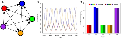
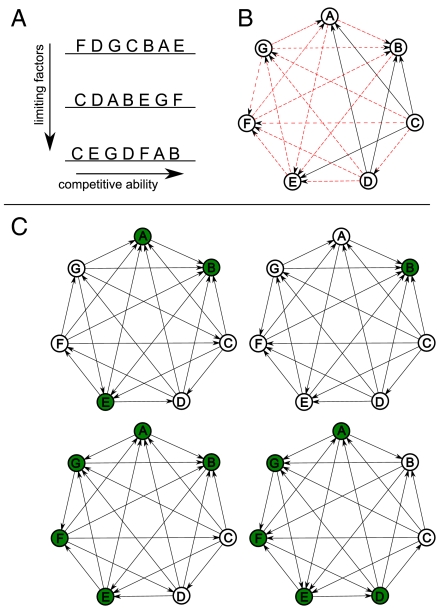
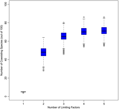
Nonhierarchical competition between species has been proposed as a potential mechanism for biodiversity maintenance, but theoretical and empirical research has thus far concentrated on systems composed of relatively few species. Here we develop a theory of biodiversity based on a network representation of competition for systems with large numbers of competitors. All species pairs are connected by an arrow from the inferior to the superior. Using game theory, we show how the equilibrium density of all species can be derived from the structure of the network. We show that when species are limited by multiple factors, the coexistence of a large number of species is the most probable outcome and that habitat heterogeneity interacts with network structure to favor diversity.

Fig. 1.

(A) Species’ competitive abilities can be represented in a tournament in which we draw an arrow from the inferior to the superior competitor for all species pairs. A tournament is a directed graph composed by n nodes (the species) connected by n(n - 1)/2 edges (arrows). (B) Simulations of the dynamics for the tournament. The simulation begins with 25,000 individuals assigned to species at random (with equal probability per species). At each time step, we pick two individuals at random and allow the superior to replace the individual of the inferior. We repeat these competitions 10⁷ times, which generates relative species abundances that oscillate around a characteristic value (SI Text). (C) The average simulated density of each species from B (shown in lighter bars) almost exactly matches the analytic result obtained using linear programming (shown in darker bars).

Fig. 2.

(A) The competitive abilities of species A–G are ranked at random for three limiting factors. (B) Two possible competitive relationships can emerge: (i) The inferior species is ranked lower than its competitor for all three factors (e.g., C versus B, black arrows) or (ii) the inferior species is ranked lower than its competitor for two factors (e.g., A and B, red arrows). (C) We can use this information to “draw” tournaments: We draw an arrow from node i to j with a probability equal to the proportion of factors for which species i is ranked below j. For example, we draw the arrow A → B with probability 2/3, whereas B → A with probability 1/3. In this way we can generate several tournaments from the same set of competitive relationships in A. For each tournament, we can find the equilibrium solution, and those species with nonzero equilibrium densities coexist (in green), though the equilibrium is neutrally stable.

Fig. 3.

Average number of species coexisting (± 1 SD) when we perform the simulations described in the main text for a variable number of limiting factors (x axis) and size of the species pool (colors). The blue line is for a 10 species pool, the red line for 20 species, and the green line for 30 species. Dashed lines mark the theoretical expectation for an infinite number of factors. (Left to Right) (A) results obtained drawing the ranking for the species independently; (B) positive correlation among factors; (C) trade-off among factors. Details are reported in SI Text.

Fig. 4.

The number of coexisting species as a function of the number of limiting factors in spatially heterogeneous systems. The simulated systems contain a pool of 100 species, competing in numerous patches, each of which is limited by a combination of up to k factors of five total factors. For example, the far left box shows the number of coexisting species in the system when each patch is limited by only one of the five factors (SI Text).

References

1. Hutchinson GE. The paradox of the plankton. Am Nat. 1961;95:137–141.
1. Gause GF. The Struggle for Existence. New York: Hafner Press; 1934. - PubMed
1. Hubbell SP. The Unified Neutral Theory of Biodiversity and Biogeography. Princeton, NJ: Princeton Univ Press; 2001. - PubMed
1. Chave J. Neutral theory and community ecology. Ecol Lett. 2004;7:241–253.
1. Alonso D, Etienne R, McKane A. The merits of neutral theory. Trends Ecol Evol. 2006;21:451–457. - PubMed
Publication types