A topological map of the compartmentalized Arabidopsis thaliana leaf metabolome

Abstract

Background: The extensive subcellular compartmentalization of metabolites and metabolism in eukaryotic cells is widely acknowledged and represents a key factor of metabolic activity and functionality. In striking contrast, the knowledge of actual compartmental distribution of metabolites from experimental studies is surprisingly low. However, a precise knowledge of, possibly all, metabolites and their subcellular distributions remains a key prerequisite for the understanding of any cellular function.

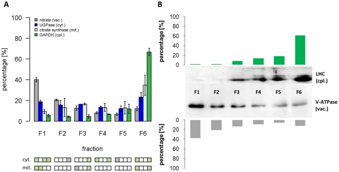
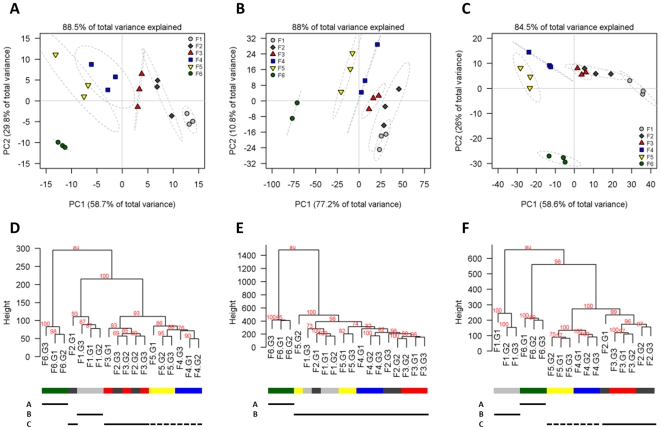
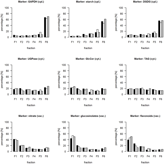
Methodology/principal findings: Here we describe results for the subcellular distribution of 1,117 polar and 2,804 lipophilic mass spectrometric features associated to known and unknown compounds from leaves of the model plant Arabidopsis thaliana. Using an optimized non-aqueous fractionation protocol in conjunction with GC/MS- and LC/MS-based metabolite profiling, 81.5% of the metabolic data could be associated to one of three subcellular compartments: the cytosol (including the mitochondria), vacuole, or plastids. Statistical analysis using a marker-'free' approach revealed that 18.5% of these metabolites show intermediate distributions, which can either be explained by transport processes or by additional subcellular compartments.

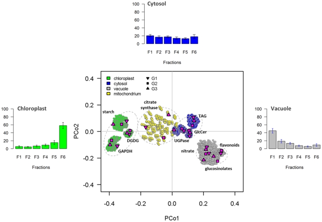
Conclusion/significance: Next to a functional and conceptual workflow for the efficient, highly resolved metabolite analysis of the fractionated Arabidopsis thaliana leaf metabolome, a detailed survey of the subcellular distribution of several compounds, in the graphical format of a topological map, is provided. This complex data set therefore does not only contain a rich repository of metabolic information, but due to thorough validation and testing by statistical methods, represents an initial step in the analysis of metabolite dynamics and fluxes within and between subcellular compartments.

Figure 1. Distribution of compartment-specific markers in non-aqueous gradients from Arabidopsis thaliana leaves.

(A) The distribution of vacuolar (nitrate), cytosolic (UGPase), mitochondrial (citrate synthase), and plastidic (GAPDH) markers are shown as the average of three independent gradients. The mean values and standard deviations of marker enzyme activities (UGPase, citrate synthase, GAPDH) or relative concentrations (nitrate) in each fraction are depicted as percentage from total (scaled data). Significant differences (P _BH<0.05, Benjamini-Hochberg corrected) using t-test within each fraction compared to the cytosolic (cyt.) or mitochondrial (mit.) marker are shown as green colored boxes below the graph. Grey boxes illustrate uncorrected significant (P<0.05) differences. (B) Western blots detecting LHC (plastidic) and vacuolar H⁺-ATPase (vacuolar) membrane proteins in each fraction are shown for one representative gradient to confirm the distribution of the plastidic and vacuolar compartment throughout the gradients. The pixel intensities quantified using ImageJ (http://rsb.info.nih.gov/ij) are drawn as bar diagrams.

Figure 2. Principal component (PCA; A–C) and hierarchical cluster (HCA; D–F) analyses of metabolite data.

Both PCA and HCA plots demonstrate a good separation of the six fractions from each other independent of the three major compound classes, (A, D) primary, (B, E) lipophilic and (C, F) secondary metabolites. PCA and HCA were performed on scaled data. For PCA, data were additionally log₂-transformed; HCA analyses are based on Euclidean distances among samples. Identical gradient fractions are encoded with the same color and shape as depicted in the graph legend. The 95% confidence ellipse is drawn as a grey dotted line on the basis of the mean, standard deviation, and correlation of the three independent gradient replicates per fraction. To aid interpretation of HCA graphs (D–F) same fractions are identically color-coded (see PCA legend) at the bottom sidebar. The unbiased cluster P-values, calculated using multiscale bootstrap resampling, are depicted as red-colored numbers at each node. The fraction groups explaining the highest variance of data and revealing a good cohesion within and separation among assigned fractions are depicted at the bottom of the HCA plots. Fraction groups, evaluated using resampling and gap statistic, were assembled by sequential merging of neighboring sample clusters with fractions assigned using membership majority voting (Figure S1). All graphs clearly support that the plastidic enriched, lowest density fraction F6 (group A) and to a lesser extent the vacuolar enriched, most dense fraction F1 are separated from the intermediately-dense fractions F2 to F5, even though for primary and secondary metabolite data two less-well separated fraction groups (F2–F3 and F4–F5) can be assumed (solid and dotted line; Figure S1).

Figure 3. Side-by-side bar plots of marker distribution representing the same subcellular compartment throughout the three independent gradients.

For all graphs scaled data were used. Marker names are provided as graph headers including the compartmental representation, i.e. cpl. - plastidic, vac. - vacuolar, and cyt. – cytosolic compartment. The bars are colored as follows: gradient 1 - black, gradient 2 – white, and gradient 3 – grey. For DGDG (cpl.), GlcCer (cyt.), TAG (cyt.), glucosinolates (vac.), and flavonoids (vac.) the abundance per fraction is based on the robust average of multiple analytes representing the individual compound class (Data S4).

Figure 4. Consistency and robustness of compartmental separation within and between gradients.

Manhattan distances among markers for each gradient were converted into a principal coordinates (PCo) space using classical multidimensional scaling (CMD) for the three independent and 729 non-redundant combinations of randomly assembled gradients. Shapes colored in magenta show the data points for the three independent gradients (G1, G2, and G3 as depicted in the figure) of each selected marker. Data points from simulated gradients are depicted as circles with coloration according to the individual compartments: green – chloroplasts, blue – cytosol, and grey – vacuole. For each compartment the 95% confidence ellipse is drawn as a dashed grey line on the basis of the mean, standard deviation, and correlation of the 729 non-redundant gradient combinations. The mitochondrial compartment (yellow circles) shows an overlapping distribution with the cytosol where the majority of data are in between the plastidic and cytosolic compartments. The principal coordinates 1 and 2 explain together in average about 96.7% of the total variance of the underlying distance matrices. For each of the three resolved compartments the distribution of average abundances including their standard deviations throughout the three independent gradients is depicted as bar plots.

Figure 5. Diagnostic plots showing the differences in estimated subcellular distributions using (A) BFA and NNLS algorithm on the three independent gradients, and (B) using BFA algorithm on the three independent and 729 simulated gradients.

The difference versus average plot (left) shows the differences (D) in dependence of the averages (A) of estimated subcellular distributions in a compartment (C, estimated as percentage) between two computational strategies (S): D_i = C_{i [S1]} – C_{i [S2]}, and A_i = 0.5 x (C_{i [S1]} + C_{i [S2]}). The corresponding computational strategies depicted in the plots are for (A) S1 = BFA and S2 = NNLS solutions, and for (B) S1 = 3 (GRD) and S2 = 729 (SIM) gradients. The histogram plot (right) shows the distribution of the M values in 1% intervals with blue solid lines indicating the 2.5% and 97.5% quantiles (95% range of observed differences). For all comparisons the average of estimated subcellular distributions (based on 3 or 729 gradients) are used.

Figure 6. Manually constructed classification tree for the partitioning of analytes into compartments and intermediate units based on their estimated subcellular distribution as well as compartmental abundance and variability.

The classification tree was used to assign an analyte into a group defining its subcellular distribution type (type) and an associated mode (mode) which represents one of the resolved compartments or the overlap between them. Assignments are based on the mean and standard deviations of the subcellular distribution, estimated using the best fit algorithm (BFA), for each analyte based on the three independent gradient data. Analytes with insufficiently explained subcellular distributions according to the selected compartment-specific markers are accounted as unexplained and are not further considered in this tree. Analytes revealing sufficiently explained fits are accounted as ‘shared’ if the minimum of the percentage value (min  =  mean - SD) in the most abundant compartment is overlapping with the maximum percentage value (max  =  mean + SD) of any other considered compartment. The corresponding mode is defined by the overlapping compartments regarding the most abundant compartment. Analytes are considered ‘specific’ with the mode according to the estimated most abundant compartment, if the minimum of the most abundant compartment is ≥75% and the values of all other (low abundant) compartments are negligible, i.e. ≤10%. If the minimum in the most abundant compartment is larger than the sum of the maxima among the other compartment and ≥66.67% (2/3 compartments), analytes are accounted as ‘dominantly’ distributed in the respective compartment. Analytes are accounted as ‘enriched’ in a compartment, if the value of the most abundant fraction is ≥50% than the sum of the other compartment. If none of this decisions result in an assignment the analyte is considered as being shared but with enrichment in a particular compartment (‘shared*’).

Figure 7. A topological map of the compartmentalized Arabidopsis thaliana leaf metabolome for (A) all and (B) selected analytes.

The classification for the partitioning of analytes into compartments and intermediate units is based on the best fit - estimated subcellular distribution as well as compartmental abundance and variability for each analyte (for details see Figure 6). The topological map (cf. Data S6 for single analytes) of the classification results for (A) all and (B) selected metabolites is visualized in principal coordinates (PCo) space on the basis of averaged Manhattan distances among analytes for the three independent gradients. To aid interpretation, analytes of the classes ‘specific’ and ‘dominant’ were both assigned into the respective compartment and color-coded accordingly: green – chloroplast, blue – cytosol, and grey – vacuole. Analytes assigned as being shared between two compartments are color coded as depicted in the figure. With exception of analytes with insufficiently explained (unexplained) subcellular distributions, all other analytes not belonging to one of the above-mentioned classes are defined as ‘others’.

Figure 8. Scatter and distribution plots of analytes with compartment-specific and unresolved subcellular distributions.

Analytes with compartment-specific distributions were identified using a classification tree based assignment (Figure 6). Analytes with insufficiently explained subcellular distribution were grouped according to k-medoids clustering (Figure S4A). For visualization, Manhattan distances among analytes for each of the three independent gradients were averaged and then converted into a principal coordinates (PCo) space. Analytes were color-coded according to their cluster membership. For each identified cluster the distribution of members throughout the gradients (grey lines) and the robust average distribution including standard deviations (black lines) are depicted as line plots. Despite the overlap of the intermediate clusters with the resolved compartments, recurring and stable distribution patterns have been observed.

References

1. Linka N, Weber AP. Intracellular metabolite transporters in plants. Mol Plant. 2010;3:21–53. - PubMed
1. Weber AP, Fischer K. Making the connections–the crucial role of metabolite transporters at the interface between chloroplast and cytosol. FEBS Lett. 2007;581:2215–2222. - PubMed
1. Martinoia E, Maeshima M, Neuhaus HE. Vacuolar transporters and their essential role in plant metabolism. J Exp Bot. 2007;58:83–102. - PubMed
1. Stitt M, Fernie AR. From measurements of metabolites to metabolomics: an ‘on the fly’ perspective illustrated by recent studies of carbon-nitrogen interactions. Curr Opin Biotechnol. 2003;14:136–144. - PubMed
1. Deuschle K, Chaudhuri B, Okumoto S, Lager I, Lalonde S, et al. Rapid metabolism of glucose detected with FRET glucose nanosensors in epidermal cells and intact roots of Arabidopsis RNA-silencing mutants. Plant Cell. 2006;18:2314–2325. - PMC - PubMed
Publication types