

Published Erratum
doi: 10.1007/s00221-011-2639-6.
Erratum to: Nonrenewal spike train statistics: causes and functional consequences on neural coding
Affiliations
- PMID: 21451983
- PMCID: PMC4587930
- DOI: 10.1007/s00221-011-2639-6
Item in Clipboard
Published Erratum
Erratum to: Nonrenewal spike train statistics: causes and functional consequences on neural coding
Exp Brain Res.
2011 May.
No abstract available
Figures
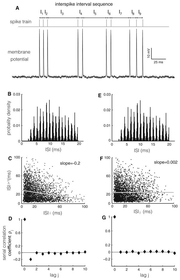
Example of nonrenewal spike train statistics. a Voltage trace from a pyramidal cell of weakly electric fish. The spike times and ISIs (I1,…I9) are also shown. It is seen that short ISIs tend to be followed by long ones and vice versa. b ISI probability distribution obtained from the same cell. c ISI return map obtained from the same cell. The slope of the best-fit line (gray) is equal to the ISI serial correlation coefficient at lag one for the spike train. d ISI serial correlation coefficients ρj as a function of lag j. Note that we have ρ1 < 0. e The ISI probability distribution obtained after randomly shuffling the ISI sequence. f The ISI return map is significantly altered by the shuffling procedure. g ISI serial correlation coefficients qj as a function of lag j for the shuffled data. Note that ρj = 0 for j > 0
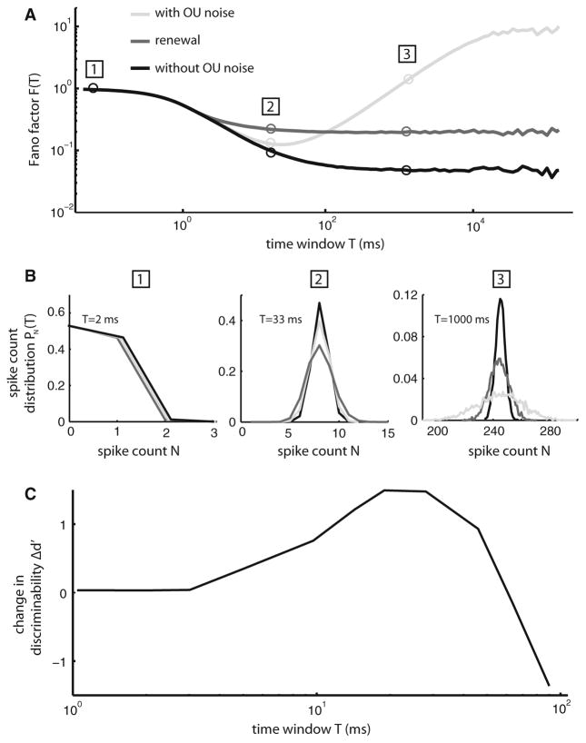
Positive and negative ISI correlations act to create a minimum in spike train variability for a given time window T. a Fano factor F(T) from the LIFDT neuron model driven by a weak Ornstein–Uhlenbeck (OU) noise with a long correlation time (light gray). Also shown are the Fano factor F(T) computed from the same model without the OU noise (black) and after shuffling the ISI sequence (dark gray). b Spike count distributions PN(T) obtained for all three conditions. For T = 2 ms (left), the distributions show almost complete overlap. However, for T = 33 ms (middle), the spike count distribution obtained from the LIFDT model without OU noise (black) shows the weakest variance, followed by the distribution obtained with the model with OU noise (light gray), followed by the distribution obtained after shuffling. However, for T = 1,000 ms (right), it is the distribution obtained from the model with OU noise (light gray) that has the highest variance. c Change in discriminability measure d′ (i.e. the difference between d′ computed from the model with OU noise and d′ computed after shuffling the ISI sequence) as a function of the time window length T. It is seen that the gain in discriminability is maximal for a value of T for which the Fano factor F(T) is minimum
Erratum for
-
Nonrenewal spike train statistics: causes and functional consequences on neural coding.Exp Brain Res. 2011 May;210(3-4):353-71. doi: 10.1007/s00221-011-2553-y. Epub 2011 Jan 26. Exp Brain Res. 2011. PMID: 21267548 Free PMC article. Review.
Publication types
Grants and funding
LinkOut - more resources
Full Text Sources
