

Review
doi: 10.1002/mrm.22924.
Epub 2011 Apr 5.
Diffusion tensor imaging and beyond
Affiliations
- PMID: 21469191
- PMCID: PMC3366862
- DOI: 10.1002/mrm.22924
Item in Clipboard
Review
Diffusion tensor imaging and beyond
Magn Reson Med.
2011 Jun.
No abstract available
Figures
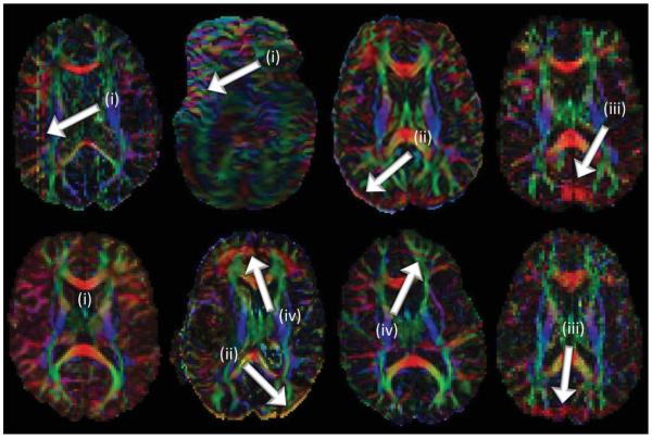
Examples of typical artifacts: (i) signal/slice dropouts, (ii) eddy-current induced geometric distortions, (iii) systematic vibration artifacts, and (iv) ghosting (insufficient/incorrect fat-suppression).
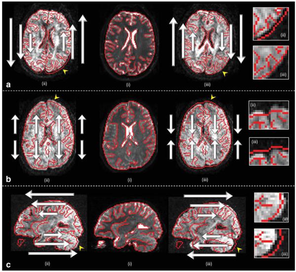
Three examples of DW images with shears, stretches, and translations induced by eddy currents in the frequency-encoded left-right (LR) direction (a), the phase-encoded anterior–posterior (AP) direction (b), and the slice-select encoded inferior–superior (IS) direction (c), respectively. For each example, the undistorted B0 image (i) is shown with lines overlaid in red indicating brain edges and boundaries of the lateral ventricles. The mismatches of these prominent contours when overlaid on the distorted DW images, shown in (ii) and (iii), now become obvious (see also the enlarged regions corresponding with the arrowheads). Notice the difference in polarity of the eddy current induced gradient between (ii) and (iii) for each example. The images in (c) are shown in a sagittal view to highlight the linearly varying image translation as a function of slice position. Note that this distortion, induced by eddy currents along the IS orientation, may be considered as a shear in the AP-IS plane.
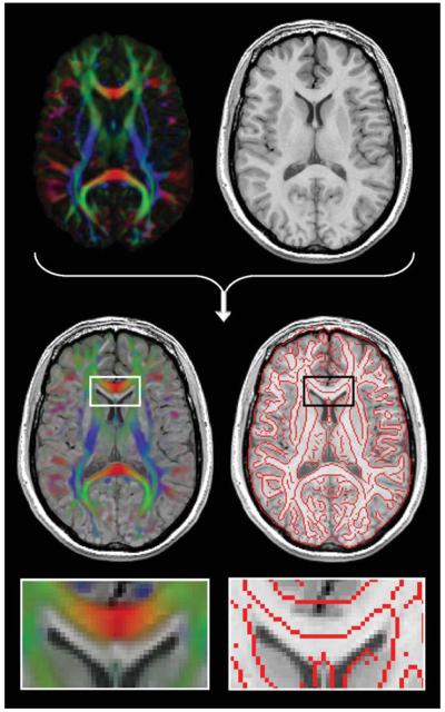
Static geometric deformations in the phase-encoded direction by B0 field inhomogeneities (or susceptibility-induced off-resonance fields). The deformations are clearly visible when fused rigidly with a structural T1 weighted image (the enlarged region shows the misalignment of the genu of the corpus between the color-encoded FA image and the T1 map).
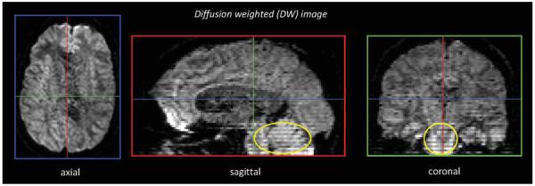
A DW image shown in three orthogonal views. The interslice instabilities (encircled) in this axially interleaved acquisition might not be seen on the axial slices, but are very prominent on the sagittal and coronal through-plane views.
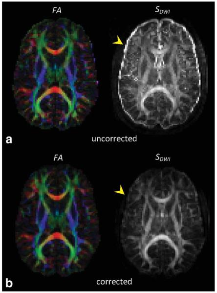
To assess subject motion, or more generally, misalignment between the DW images, computing the standard deviation across the DW images SDWI is an efficient and more quantitative approach than inspection of the DW images on a slice-by-slice basis. The bright rim in the SDWI map shown in (a) is not present after correction for subject motion and eddy current induced geometric distortions (b) (see arrowheads).
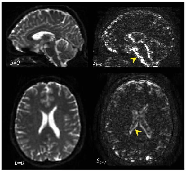
In the b = 0 images (i.e., the non-DWIs), unreliable regions in terms of signal variability (most likely due to pulsation artifacts) can be visualized readily by taking the standard deviation across the b = 0 images (Sb = 0). For the example shown here, six b = 0 images were acquired. Notice the high variability near the medial parts of the brainstem, cerebellum, and the lateral ventricles.
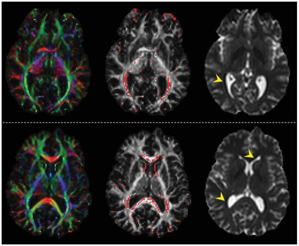
Examples of “physically implausible signals” (i.e., voxels where the B0 intensity is lower than the DW intensities) that contaminate the fractional anisotropy (FA) values. When comparing the locations of the corrupted voxels (in red) between the middle and the left image, these FA values are typically overestimated. A more detailed investigation revealed the presence of negative eigenvalues, which were caused by ill-conditioned diffusion tensor estimations. The corresponding B0 images on the right contain the artifacts (Gibbs-ringing) that formed the basis of these error accumulations: parallel to the interface between the CSF and the surrounding white matter, artificially low intensity rims can be observed (see arrowheads), which is typically seen in images with a relatively small acquisition matrix.
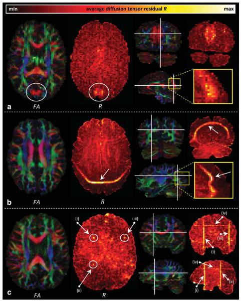
Three examples that showcase the high sensitivity of diffusion tensor residual maps (R) to detect artifacts. a: The experienced DTI user will immediately spot the phantom commissural pathways that connect left and right occipital lobes on the directionally color-encoded fractional anisotropy (FA) maps (encircled). If one is unfamiliar with the rich (colorful) information contained in these images, however, or when pathology is involved, the corresponding R map is a useful tool to differentiate between low and high quality regions. In this example, the artifact is clearly visible on the R map as well. By contrast, in (b) and (c), the artifacts, i.e., ghosting due to insufficient fat suppression and RF interference (i)–(iii)/slice dropout (iv), respectively, are not visible on the FA maps and can hardly be seen on the individual DW images themselves.
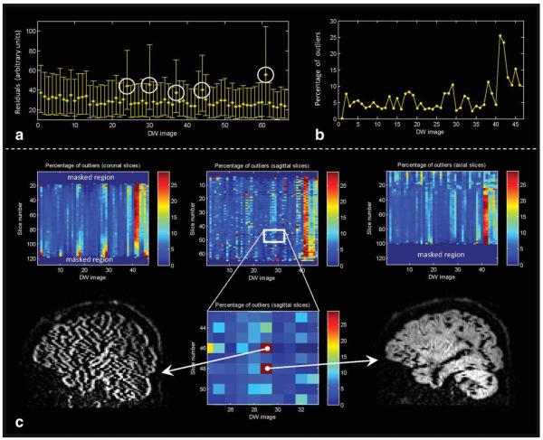
a: Diffusion tensor residuals calculated for each DW image (averaged across all brain voxels—see Eq. 3, with the error bars representing the inter-quartile range). In the example shown, five diffusion volumes were “heavily” corrupted as indicated by the higher residuals (encircled). b: A more quantitative feel of the significance of high residual values is obtained by calculating the “statistical” outliers of these tensor residuals. The percentage of outliers per DW image may then serve as a marker to identify artifacts. c: To increase the specificity of detecting artifacts, the same procedure can be applied to each slice separately and along the different (coronal, axial, and sagittal) image views. In this way, a summary statistic of data quality can be shown for each slice and for all the DW gradient directions simultaneously in a single matrix. Retrospective identification of “problematic” slices is then facilitated by the “hot spots” (see enlarged region).
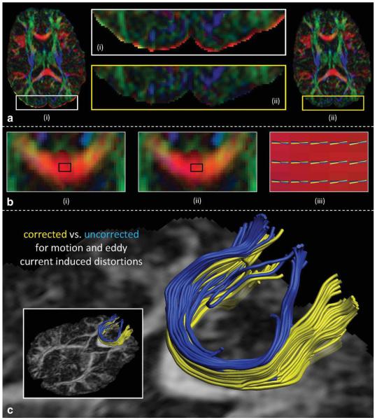
a: Directionally color-encoded fractional anisotropy (FA) maps before (i) and after (ii) correcting for subject motion and eddy current-induced geometric distortions. The bright rim (see enlarged region), clearly visible in (i), is practically nonexistent in the corrected image (ii). In this example, geometric distortions and subject motion in the DW images are corrected for simultaneously. As a result, the orientation of the diffusion gradients should be adjusted to take potential head rotations into account. In (b), the difference in orientation of the estimated first eigenvector between the uncorrected (i) and the corrected (ii) gradient directions is shown in a region of the genu. To fully appreciate the effect of neglecting this processing step, the glyph representations of the first eigenvectors are shown in (iii) (blue: uncorrected; yellow: corrected), focusing on the mid-sagittal region, which corresponds with the black rectangle in (i) and (ii). Although the errors shown in (iii) seem small and, therefore, perhaps deemed insignificant, the tractography results in (c) clearly show the deviation in the reconstructed fiber tract pathways when subject motion and eddy current-induced geometric distortions are not taken into account.
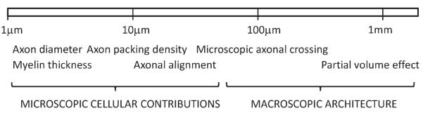
Various anatomical factors that could influence the diffusion anisotropy measurement by DTI and their approximate scale.
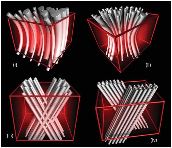
Simulated configurations of complex fiber bundle architecture at the length scale of a single voxel (61). Note that any tract organization different from a single straight fiber population is typically referred to as “crossing fibers,” including (i) bending (e.g., uncinate fasciculus) and (ii) fanning (e.g., pyramidal projections) fiber bundles. Interdigitating fibers, as shown in (iii), might occur in the region of the centrum semiovale, where the lateral projections of the corpus callosum intersect with the corticospinal tract among others. By contrast, the configuration shown in (iv) reflects adjacent fiber bundles, such as the cingulum bundle and the body of the corpus callosum, which—by definition of the partial volume effect—are captured within a single voxel.
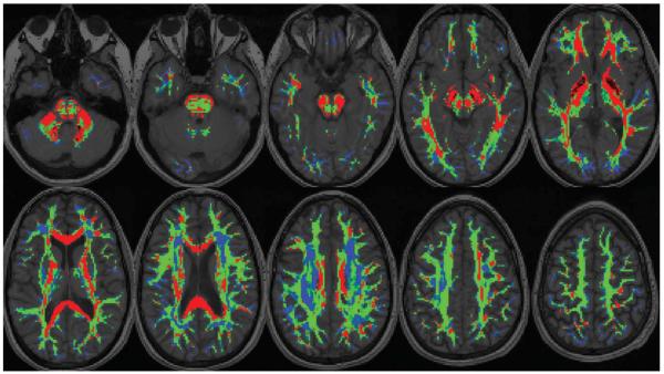
The number of distinct fiber orientations detected within each voxel (98), overlaid on the corresponding anatomical T1-weighted image. Each voxel within the mask is colored according to the number of orientations detected (red: single orientation; green: two orientations; blue: more than two orientations). These results were produced from data obtained from a healthy volunteer, consisting of 15 repeats of 30 DW directions, acquired at b = 1000 s/mm2, analyzed using constrained spherical deconvolution (99) within a “bootstrap” framework (100). Image courtesy of Ben Jeurissen.
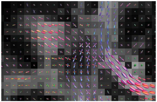
Fiber orientation distributions for each voxel, for a coronal section showing the lateral projections of the corpus callosum (left-right: red lobes) crossing through the fibers of the corona radiata (inferior–superior: blue lobes) and of the superior longitudinal fasciculus (anterior–posterior: green lobes). Results produced from data obtained from a healthy volunteer, consisting of 60 DW directions acquired at b = 3000 s/mm2 (9 min scan time), analyzed using constrained spherical deconvolution (99).
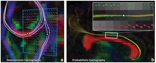
Conceptual example of (a) deterministic (Ref. 20) and (b) probabilistic (Ref. 145) streamline tractography based on the diffusion tensor model. The white lines in (a) represent fiber tract pathways that were reconstructed by following the principal diffusion directions (see the glyphs shown in the blue region of interest) in consecutive steps, initiated bidirectionally at the indicated locations (i.e., “seed points”). For each of the pathways in (a), there is no information available about the precision/dispersion that is associated with their tract propagation. By contrast, the set of multiple (1000) lines shown in (b) provides a feel for the degree of uncertainty related to the tract reconstruction initiated from the single seed point. Note that the same underlying tractography algorithm (Ref. 20) was used for both examples, but in (b), each tract pathway was calculated from a “different” diffusion tensor data set that was created with the wild-bootstrap approach (Ref. 145).
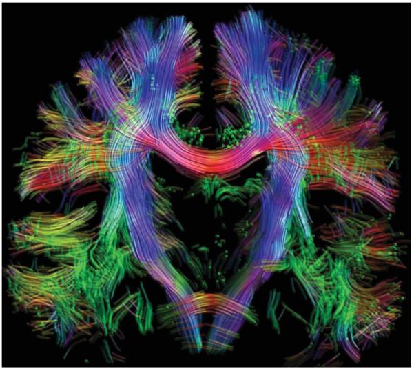
Whole-brain nontensor probabilistic tractography results displayed as a coronal 2-mm-thick section. Each track is colored according to its direction of travel (red: left–right; green: anterior–posterior; blue: inferior–superior). 100,000 tracks were produced by seeding at random throughout the brain, with a probabilistic streamlines algorithm using fiber orientation distributions estimated using constrained spherical deconvolution (99), based on the same data as shown in Fig. 8. Note in particular the extensive regions of crossing fibers in the pons and periventricular areas.
References
-
- Le Bihan D, Breton E, Lallemand D, Grenier P, Cabanis E, Laval-Jeantet M. MR imaging of intravoxel incoherent motions: application to diffusion and perfusion in neurologic disorders. Radiology. 1986;161:401–407. - PubMed
-
- Le Bihan D, Turner R, MacFall J. Effects of intravoxel incoherent motions (IVIM) in steady-state free precession (SSFP) imaging: application to molecular diffusion imaging. Magn Reson Med. 1989;10:324–337. - PubMed
-
- Merboldt KD, Bruhn H, Frahm J, Gyngell ML, Hanicke W, Deimling M. MRI of “diffusion” in the human brain: new results using a modified CE-FAST sequence. Magn Reson Med. 1989;9:423–429. - PubMed
-
- Chenevert TL, Brunberg JA, Pipe JG. Anisotropic diffusion in human white matter: demonstration with MR technique in vivo. Radiology. 1990;177:401–405. - PubMed
Publication types
MeSH terms
Grants and funding
LinkOut - more resources
Full Text Sources
Other Literature Sources
