Effective connectivity: influence, causality and biophysical modeling

Abstract

This is the final paper in a Comments and Controversies series dedicated to "The identification of interacting networks in the brain using fMRI: Model selection, causality and deconvolution". We argue that discovering effective connectivity depends critically on state-space models with biophysically informed observation and state equations. These models have to be endowed with priors on unknown parameters and afford checks for model Identifiability. We consider the similarities and differences among Dynamic Causal Modeling, Granger Causal Modeling and other approaches. We establish links between past and current statistical causal modeling, in terms of Bayesian dependency graphs and Wiener-Akaike-Granger-Schweder influence measures. We show that some of the challenges faced in this field have promising solutions and speculate on future developments.

Fig. 1

Overview of causal modeling in Neuroimaging. Overall view of conceptual framework for defining and detecting effective connectivity in Neuroimaging studies.

Fig. 2

Data and model driven approaches to causal modeling. Data driven approaches look for nonparametric models that not only fit the data but also describe important dynamical properties. They complement hypothesis driven approaches that are not only constrained by having to explain dynamical behavior but also provide links to computational models of brain function.

Fig. 3

Bayesian inference on the connectivity matrix as a random field. a) Causal modeling in Neuroimaging has concentrated on inference on neural states x(r, t) ∈ R defined on a subset of nodes in the brain. However, spatial priors can be used to extend models into the spatial domain (cf., minimum norm priors over current source densities in EEG/MEG inverse problems). b) In connectivity analysis, attention shifts to the AR (connectivity) matrix (or function) a(r, r′), where the ordered pairs (r, r′) belong to the Cartesian product R × R. For this type of inference, priors are now placed on the connectivity matrix. c) Sparse multivariate autoregression obtains by penalizing the columns of a full multivariate autoregressive model (Valdés-Sosa et al., 2005) thus forcing the columns of the connectivity matrix to be sparse. The columns of the connectivity matrix are the “outfields” that map each voxel to the rest of the brain. This is an example of using sparse (spatial) hyperpriors to regularize a very difficult inverse problem in causal modeling.

Fig. 4

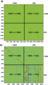
Sparse multivariate autoregression of concurrent EEG/fMRI recordings. Intra and inter modality connectivity matrix for a concurrent EEG/fMRI recordings. The data analyzed here were the time courses of the average activity in 579 ROI: for BOLD (first half of data vector) and EEG power at the alpha peak. A first-order sparse multivariate autoregressive model was fitted with an l₁ norm (hyper) prior on the coefficient matrix. The t-statistics of the autoregression coefficients where used for display. The color bar is scaled to the largest absolute value of the matrix, where green codes for zero. a) the innovation covariance matrix reflecting the absence of contemporaneous influences: b) t-statistics for the lag 1 AR coefficients.

Fig. 5

The missing region problem. a) Two typical graphical models including a hidden node (node 2).b) Marginal dependence relationships implied by the causal structure depicted in (a), after marginalizing over the hidden node 2; the same moral graph can be derived from directed (causal) graphs A and B. c) Causal relationships implied by the causal structure depicted in (a), after marginalizing over the hidden node 2. Note that these are perfectly consistent with the moral graph in (b), depicting (non causal) statistical dependencies between nodes 1 and 3, which are the same for both A and B.

Fig. 6

Wiener–Akaike–Granger–Schweder (WAGS) Influences. This figure illustrates the different types of WAGS influence measures. In the middle X₂(t) a continuous time point process, which may be influencing the differentiable continuous time process X₁(t) (top and bottom) This process may have local influence (full arrows), which indicate predictability in the immediate future (dt), or global influence (dashed arrow) at any set of future times. If predictability pertains to the whole probability distribution, this is a strong influence (bottom), and a weak influence (top) if predictability is limited to the moments (e.g., expectation) of this distribution.

Fig. 7

The missing time problem. This figure provides a schematic representation of spurious causality produced by sub-sampling. a) Three time series X₁(t), X₂(t), and X₃(t) are shown changing at an “infinitesimal” time scale with steps dt, as well as at a coarser sampled time scale with set ∆t. Each time series, influences itself at later moments. In the example X₃(t) directly influences X₂(t), with no direct influence on X₁(t). In turn X₂(t) directly influences X₁(t), with no direct influence on X₃(t). Finally X₁(t) does not influence either X₃(t) nor X₂(t). There are no contemporaneous influences. b) When only observing at the coarser time scale ∆t, spurious contemporaneous influences (mediated by intermediate nodes) appear between X₂(t) and X₁(t) and between X₃(t) and X₂(t). In addition a spurious direct influence appears between X₃(t) and X₁(t). The graphical representations of the true and spurious causal relations are to the right of each figure where an arrow represents direct influence and a double arrow represents contemporaneous influence. Estimating these spurious influences can only be avoided by explicitly modeling their effect from continuous models or using models such as VARMA models which are resistant to this phenomena.

Fig. 8

Direct and indirect effects. Causal relationships implied by the DCM given in Eq. (23). On the left the apparent graph, that includes feedback which precludes causal analysis. Note that the causal links are actually expressed through implicit delays, which makes this graph a DAG, which is seen more clearly on the right where each node is expanded at several time instants.

References

1. Aalen O.O. Dynamic modeling and causality. Scand. Actuarial J. 1987;13:177–190.
1. Aalen O.O., Frigessi A. What can statistics contribute to a causal understanding. Scand. J. Stat. 2007;34(1):155–168. doi: 10.1111/j.1467-9469.2006.00549.x. - DOI
1. Akaike H. 20(1) Springer; 1968. On the use of a linear model for the identification of feedback systems; pp. 425–439.http://www.springerlink.com/index/MP5748216213R74Q.pdf (Annals of the Institute of Statistical Mathematics). Retrieved from.
1. Amendola A., Niglio M., Vitale C. Temporal aggregation and closure of VARMA models: some new results. In: Palumbo F., Lauro C.N., Greenacre M.J., editors. Data Analysis and Classification. Springer Berlin Heidelberg; Berlin, Heidelberg: 2010. pp. 435–443. - DOI
1. Anguelova M., Wennberg B. 46(4) Elsevier Ltd.; 2010. On analytic and algebraic observability of nonlinear delay systems; pp. 682–686. (Automatica). - DOI
MeSH terms
LinkOut - more resources