Fibre operating lengths of human lower limb muscles during walking

Abstract

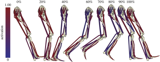
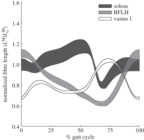
Muscles actuate movement by generating forces. The forces generated by muscles are highly dependent on their fibre lengths, yet it is difficult to measure the lengths over which muscle fibres operate during movement. We combined experimental measurements of joint angles and muscle activation patterns during walking with a musculoskeletal model that captures the relationships between muscle fibre lengths, joint angles and muscle activations for muscles of the lower limb. We used this musculoskeletal model to produce a simulation of muscle-tendon dynamics during walking and calculated fibre operating lengths (i.e. the length of muscle fibres relative to their optimal fibre length) for 17 lower limb muscles. Our results indicate that when musculotendon compliance is low, the muscle fibre operating length is determined predominantly by the joint angles and muscle moment arms. If musculotendon compliance is high, muscle fibre operating length is more dependent on activation level and force-length-velocity effects. We found that muscles operate on multiple limbs of the force-length curve (i.e. ascending, plateau and descending limbs) during the gait cycle, but are active within a smaller portion of their total operating range.

Figure 1.

Three-dimensional musculoskeletal model of the lower limb during one gait cycle. Bony geometry includes the phalanges, metatarsals, calcaneus, talus, fibula, tibia, patella, femur and pelvis. Joint angles and angular velocities were calculated for 10 gait cycles and then averaged over a common basis of 0–100% to produce one characteristic gait cycle beginning and ending at heel strike. Muscle-tendon actuators representing lower limb muscles were constrained to origin and insertion points and wrapping surfaces. Typical muscle activation patterns for walking were prescribed for each muscle on a 0.00 to 1.00 scale, representing 0 to 100% activation.

Figure 2.

Lumped parameter model of muscle used to simulate tendon and muscle dynamics [5]. (a) The muscle–tendon length (L^MT) derived from the muscle–tendon geometry was used to compute muscle fibre length (L^M), fibre shortening velocity (v^M), tendon length (L^T), pennation angle (α), muscle force (F^M) and tendon force (F^T). Muscle was represented as a passive elastic element in parallel with an active contractile element (CE). Tendon was represented as a nonlinear elastic element. 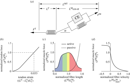(b) Tendon force–strain relationship assumed that the strain in tendon () was 0.033 when the muscle generated maximum isometric force (). 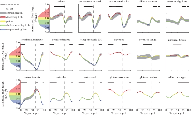(c) Normalized active and passive force–length curves were scaled by maximum isometric force () and optimal fibre length () derived from experimental measurements for each muscle. The regions of the active force–length curve were described as the steep ascending limb (blue), shallow ascending limb (green), plateau (yellow) and descending limb (red). (d) The force–velocity curve included concentric (v^M > 0) and eccentric (v^M < 0) regions and was scaled by maximum isometric force and .

Figure 3.

Joint angles prescribed for the simulation. The kinematics of the subject's characteristic gait cycle (solid lines) were calculated as the average of 10 consecutive gait cycles. These joint angles were compared with those reported by Kadaba et al. [40], ±1 s.d., which were adjusted so that the timing of toe-off (dashed line) aligned with our subject (shaded region). Joint angles were comparable with some discrepancies owing to variation in the definitions of joint angles and coordinate frames.

Figure 4.

Feasible operating region of normalized fibre length for soleus, BFLH and vastus lateralis during one gait cycle. For the prescribed joint angles, any activation pattern will produce a trajectory of normalized fibre length in this range. The feasible operating region for each muscle is the difference between fibre length trajectories during gait for minimum and maximum activation. Muscles with long tendons relative to their optimal fibre length (i.e. large values of ) have wider feasible operating ranges than muscles with relatively short tendons.

Figure 5.

Effect of force–velocity property on trajectory of normalized fibre length in medial gastrocnemius. Increased force in eccentric contraction and decreased force in concentric contraction, compared with isometric contraction, alter tendon strain. As a result, normalized fibre length calculated with a dynamic simulation (solid line) was shorter in eccentric contraction and longer in concentric contraction than would be determined from a static calculation (dashed line).

Figure 6.

Trajectory of normalized fibre length, feasible operating region and the period of activation during gait for 17 lower limb muscles. The feasible operating regions (grey) were calculated for minimum to maximum activation. Trajectories of normalized fibre length were calculated for the activation pattern reported by Winter [43] (solid, multi-coloured line). The colours of the curve correspond to the limbs of the force–length curve shown on the far left of each row. Portions of the gait cycle when a muscle's activation exceeded its mean value for the gait cycle are indicated at the top of each plot (thick black line). Toe-off is indicated at 66% (dashed line).

Figure 7.

Effect of tendon stiffness on trajectory of normalized fibre length and feasible operating region. The default tendon force–strain relationship was altered in soleus so that the tendon was half as stiff (i.e., tendon strain was 0.066 at peak isometric muscle force). Compared to the default operating region (dotted area) and trajectory of normalized fibre length (dashed line) modelling soleus with half the tendon stiffness reduces the lower limit of the operating region (grey area) and produces shorter, more isometric fibre length (solid line) when the muscle is active.

References

1. Gordon A. M., Huxley A. F., Julian F. J. 1966. The variation in isometric tension with sarcomere length in vertebrate muscle fibres. J. Physiol. 184, 170–192 - PMC - PubMed
1. Magid A., Law D. J. 1985. Myofibrils bear most of the resting tension in frog skeletal muscle. Science 230, 1280–128210.1126/science.4071053 (doi:10.1126/science.4071053) - DOI - DOI - PubMed
1. Bahler A. S., Fales J. T., Zierler K. L. 1968. The dynamic properties of mammalian skeletal muscle. J. Gen. Physiol. 51, 369–38410.1085/jgp.51.3.369 (doi:10.1085/jgp.51.3.369) - DOI - DOI - PMC - PubMed
1. Joyce G. C., Rack P. M. 1969. Isotonic lengthening and shortening movements of cat soleus muscle. J. Physiol. 204, 475–491 - PMC - PubMed
1. Zajac F. E. 1989. Muscle and tendon: properties, models, scaling, and application to biomechanics and motor control. Crit. Rev. Biomed. Eng. 17, 359–411 - PubMed
Publication types