Origin and diversification dynamics of self-incompatibility haplotypes

Abstract

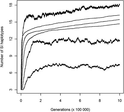
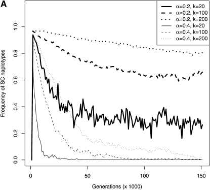
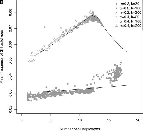
Self-incompatibility (SI) is a genetic system found in some hermaphrodite plants. Recognition of pollen by pistils expressing cognate specificities at two linked genes leads to rejection of self pollen and pollen from close relatives, i.e., to avoidance of self-fertilization and inbred matings, and thus increased outcrossing. These genes generally have many alleles, yet the conditions allowing the evolution of new alleles remain mysterious. Evolutionary changes are clearly necessary in both genes, since any mutation affecting only one of them would result in a nonfunctional self-compatible haplotype. Here, we study diversification at the S-locus (i.e., a stable increase in the total number of SI haplotypes in the population, through the incorporation of new SI haplotypes), both deterministically (by investigating analytically the fate of mutations in an infinite population) and by simulations of finite populations. We show that the conditions allowing diversification are far less stringent in finite populations with recurrent mutations of the pollen and pistil genes, suggesting that diversification is possible in a panmictic population. We find that new SI haplotypes emerge fastest in populations with few SI haplotypes, and we discuss some implications for empirical data on S-alleles. However, allele numbers in our simulations never reach values as high as observed in plants whose SI systems have been studied, and we suggest extensions of our models that may reconcile the theory and data.

Figure 1.—

Limits of the regions where the different evolutionary outcomes are observed, for an initial number of S haplotypes n = 5. (A) In an infinite population: solid lines are the results of the stability analysis (thick line, fate of the pollen-part mutant S_b when it is frequent; thin line, evolutionary outcome when S_b is rare; see text for further details). The dashed line limit was obtained through numerical iterations and delimits the region where haplotype S_n was not excluded after the introduction of the pollen-part mutant S_b. Diamonds refer to the parameters that we investigated to approximate this limit. We define four regions according to which haplotypes are excluded when S_b is introduced at low frequency in the population. These four regions are the loss region (L), when the pollen-part mutant S_b goes to fixation; the replacement region (R), when only S_n is excluded; the maintenance regions (M1 + M2), when S_b alone is excluded; and the diversification regions (D1 + D2), when no haplotypes are excluded, and a new S haplotype can emerge. (B) In a finite population (N = 5000, μ = 5 × 10⁻⁷, k = 20): we defined four regions according to which evolutionary outcome was the most frequent in our simulations for a given set of parameters: the loss region (L, where loss of the SI system was mainly observed), the polymorphism region (P, where the populations were composed of a mix of SC and SI haplotypes), the maintenance region (M, where only SI haplotypes were observed and the number of specificities did not increase), and the diversification region (D, where no SC haplotypes were observed and the number of SI haplotypes increased).

Figure 1.—

Limits of the regions where the different evolutionary outcomes are observed, for an initial number of S haplotypes n = 5. (A) In an infinite population: solid lines are the results of the stability analysis (thick line, fate of the pollen-part mutant S_b when it is frequent; thin line, evolutionary outcome when S_b is rare; see text for further details). The dashed line limit was obtained through numerical iterations and delimits the region where haplotype S_n was not excluded after the introduction of the pollen-part mutant S_b. Diamonds refer to the parameters that we investigated to approximate this limit. We define four regions according to which haplotypes are excluded when S_b is introduced at low frequency in the population. These four regions are the loss region (L), when the pollen-part mutant S_b goes to fixation; the replacement region (R), when only S_n is excluded; the maintenance regions (M1 + M2), when S_b alone is excluded; and the diversification regions (D1 + D2), when no haplotypes are excluded, and a new S haplotype can emerge. (B) In a finite population (N = 5000, μ = 5 × 10⁻⁷, k = 20): we defined four regions according to which evolutionary outcome was the most frequent in our simulations for a given set of parameters: the loss region (L, where loss of the SI system was mainly observed), the polymorphism region (P, where the populations were composed of a mix of SC and SI haplotypes), the maintenance region (M, where only SI haplotypes were observed and the number of specificities did not increase), and the diversification region (D, where no SC haplotypes were observed and the number of SI haplotypes increased).

Figure 2.—

Effect of the initial number of specificities (n) on the different evolutionary outcomes in an infinite population. Solid and dashed lines define the limits of each region (L, R, M1, M2, D1, and D2; see Figure 1 legend). The diversification region is indicated at the top for the different n’s. Note that some diversification regions are overlapping. The area of the diversification region decreased when n increased, except for n = 3 and n = 4. The diversification region was also displaced toward smaller values of δ and α when n increased. Stars indicate the values of δ and α that were chosen to investigate the diversification dynamics across 10⁶ generations in Figure 4.

Figure 3.—

The diversification region in a finite population for different population sizes and mutation rates, with an initial number of specificities n = 5. Grid cells are figured in shades of gray that are proportional to the number of simulations where diversification was observed (n > 5 at the end of the simulation), with black squares corresponding to sets of parameters under which the evolutionary outcome was only diversification and white squares corresponding to cases under which no diversification was observed. One hundred replicate runs were performed for each combination of parameter values (population size N, mutation rate μ). k = 20 for all simulations.

Figure 4.—

Diversification dynamics in finite populations across 10⁶ generations. The number of SI haplotypes in the population was averaged over 100 replicates. Simulations were performed with N = 5000, μ = 5 × 10⁻⁵, δ = 0.9, the initial number of SI haplotypes n = 3, and for three different values of the maximum number of specificities (k) and two values of the proportion of self-pollen (α). Thick line, α = 0.2; thin line, α = 0.4. For a given α, curves correspond to k = 20, 100, and 200 from top to bottom.

Figure 5.—

Genotypic composition of the population in the first 150,000 generations to investigate the dynamics of birth and death of SI haplotypes (genotypic frequencies sampled every 1000 generations in 20 replicates for N = 5000, μ = 5 × 10⁻⁵, and δ = 0.9). (A) Mean cumulated frequency of all SC haplotypes as a function of time. After an initial rapid increase in the total frequency of SC haplotypes, their frequency started to decrease as the number of SI haplotypes increased (see Figure 4). (B) Mean frequency of SI haplotypes as a function of their total number. Symbols are mean frequencies in simulations and lines are the expected frequencies at deterministic equilibrium in an infinite population (computed using equations in Appendix A1. Pollen-part mutation with a frequency of S_n, p_n = 0 and setting n = x + 1 when x SI haplotypes were segregating within the population). For both values of α, the mean frequency of SI haplotypes increased with their total number. This is due to the fact that when the number of SI haplotypes increases, the total frequency of SC haplotypes decreases, thus leaving a larger range of frequency for SI haplotypes. When α = 0.4, the mean frequency of SI haplotypes decreased when their number was >12 because the frequency of SC haplotypes approached zero. There was no similar threshold value of the number of SI haplotypes in the case α = 0.2 because the frequency of SC haplotypes remained high.

Figure 5.—

Genotypic composition of the population in the first 150,000 generations to investigate the dynamics of birth and death of SI haplotypes (genotypic frequencies sampled every 1000 generations in 20 replicates for N = 5000, μ = 5 × 10⁻⁵, and δ = 0.9). (A) Mean cumulated frequency of all SC haplotypes as a function of time. After an initial rapid increase in the total frequency of SC haplotypes, their frequency started to decrease as the number of SI haplotypes increased (see Figure 4). (B) Mean frequency of SI haplotypes as a function of their total number. Symbols are mean frequencies in simulations and lines are the expected frequencies at deterministic equilibrium in an infinite population (computed using equations in Appendix A1. Pollen-part mutation with a frequency of S_n, p_n = 0 and setting n = x + 1 when x SI haplotypes were segregating within the population). For both values of α, the mean frequency of SI haplotypes increased with their total number. This is due to the fact that when the number of SI haplotypes increases, the total frequency of SC haplotypes decreases, thus leaving a larger range of frequency for SI haplotypes. When α = 0.4, the mean frequency of SI haplotypes decreased when their number was >12 because the frequency of SC haplotypes approached zero. There was no similar threshold value of the number of SI haplotypes in the case α = 0.2 because the frequency of SC haplotypes remained high.

References

1. Billiard S., Lopez-Villavicencio M., Devier B., Hood M., Fairhead C., Giraud T., 2011. Having sex, yes, but with whom? Inferences from fungi on the evolution of anisogamy and mating types. Biol. Rev. 86: 421–442 - PubMed
1. Castric V., Vekemans X., 2007. Evolution under strong balancing selection: how many codons determine specificity at the female self-incompatibility gene SRK in Brassicaceae. BMC Evol. Biol. 7: 132. - PMC - PubMed
1. Castric V., Bechsgaard J. S., Grenier S., Noureddine R., Schierup M. H., et al. , 2010. Molecular evolution within and between self-incompatibility specificities. Mol. Biol. Evol. 27: 11–20 - PubMed
1. Charlesworth D., 2000. How can two-gene models of self-incompatibility generate new specificities? Plant Cell 12: 309–310 - PMC - PubMed
1. Charlesworth D., Charlesworth B., 1979. Evolution and breakdown of S-allele systems. Heredity 43: 41–55