Switching processes in financial markets

Abstract

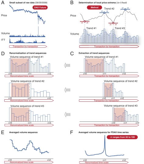
For an intriguing variety of switching processes in nature, the underlying complex system abruptly changes from one state to another in a highly discontinuous fashion. Financial market fluctuations are characterized by many abrupt switchings creating upward trends and downward trends, on time scales ranging from macroscopic trends persisting for hundreds of days to microscopic trends persisting for a few minutes. The question arises whether these ubiquitous switching processes have quantifiable features independent of the time horizon studied. We find striking scale-free behavior of the transaction volume after each switching. Our findings can be interpreted as being consistent with time-dependent collective behavior of financial market participants. We test the possible universality of our result by performing a parallel analysis of fluctuations in time intervals between transactions. We suggest that the well known catastrophic bubbles that occur on large time scales--such as the most recent financial crisis--may not be outliers but single dramatic representatives caused by the formation of increasing and decreasing trends on time scales varying over nine orders of magnitude from very large down to very small.

Fig. 1.

Segregation and rescaling of trend sequences in a multivariate time series in order to analyze financial market quantities on the path from one price extremum to the next. (A) Small subset comprising 121,400 transactions of the full dataset (13,991,275 transactions) analyzed, extracted from the German DAX future (FDAX) time series which provides transaction prices, transaction volumes, and time intervals between transaction—intertransaction times (ITT). This subset recorded on September 29, 2008 documents the volatile reaction of stock markets as the US government’s $700 billion financial bailout plan was rejected by the House of Representatives on that day. (B) Schematic visualization of trend segregation for Δt = 3. Positive trends start at local price minima (red circles) and end at local maxima (blue circle)—and vice versa. A transaction price p(t) is a local maximum if there is no higher transaction price in the interval t - Δt ≤ t ≤ t + Δ. Analogously, p(t) is a local minimum if there is no lower transaction price in the interval t - Δt ≤ t ≤ t + Δ. (C) Segregated sequences of transaction volumes belonging to the three trends identified in (B). We assign ε = 0 to the start of each trend, and ε = 1 to the end of each trend. In order to study trend switching processes—both before as well as after the end of a trend—we consider additionally the subsequent volume sequences of identical length. (D) Visualization of the volume sequences in the renormalized time scale. The renormalization assures that trends of various lengths can be aggregated as all switching points have a common position in this renormalized scale. (E) Averaged volume sequence derived from the summation of the three trend sequences. (F) Average volume sequence v^∗(ε) for all trends in the full FDAX time series derived from summation over various values of Δt. Extreme values of the price coincide with peaks in the time series of the volumes.

Fig. 2.

Renormalization time analysis and log–log plots of quantities with scale-free properties. (A) Averaged volume sequence v^∗(ε) of the German DAX Future time series. Δt ranges from 50 to 100 transactions (ticks). Extreme values of the price coincide with sharp peaks in the volume time series. (B) A very similar behavior is obtained for the averaged volume sequence v^∗(ε) of S&P500 stocks. Here, Δt ranges from 10 days to 100 days. (C) Averaged intertrade time sequence τ^∗(ε) of the German DAX Future time series. Extreme values of the price time series are reached with a significant decay of intertrade times (50 ticks ≤ Δt ≤ 100 ticks). Averaged volume and averaged intertrade time sequences are asymmetric for two main reasons: Only ε = 0 and ε = 1 correspond to extreme values in the price time series. In order to study the behavior before and after a trend switching point, we extend individual sequences from ε = 0 to ε = 1 by an identical amount of transactions or intertrade times. In addition, the end of a trend, ε = 1, does not necessarily correspond to the starting point of the next trend due to filter criteria mentioned in the main text. (D) Log—log plot of the FDAX transaction volumes (50 ticks ≤ Δt ≤ 1,000 ticks) before reaching an extreme price value (ε < 1, circles) and after reaching an extreme price value (ε > 1, triangles). 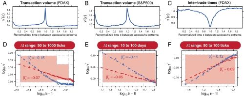The straight lines correspond to power-law scaling with exponents (t-test, p-value = 9.2 × 10^-16) and (t-test, p-value < 2 × 10^-16). The shaded intervals mark the region in which the empirical data are consistent with a power-law behavior. The left border of the shaded regions is given by the first measuring point closest to the switching point. The right borders stem from statistical tests of the power-law hypothesis (see SI Appendix). (E) Log—log plot of the transaction volumes shown in (B) indicates a power-law behavior with exponents (t-test, p-value < 2 × 10^-16) and (t-test, p-value = 1.7 × 10^-9) which are similar to our results on short time scales. (F) Log—log plot of the intertrade times on short time scales (50 ticks ≤ Δt ≤ 100 ticks) exhibits a power-law behavior with exponents (t-test, p-value < 2 × 10^-16) and (t-test, p-value = 1.8 × 10^-15). An equivalent analysis on long time scales is not possible as daily closing prices are recorded with equidistant time steps.

References

-
- Axtell RL. Zipf distribution of U.S. firm sizes. Science. 2001;293:1818–1820. - PubMed
- Stanley MHR, et al. Zipf plots and the size distribution of firms. Economics Letters. 1995;49:453–457.
- Gabaix X, Gopikrishnan P, Plerou V, Stanley HE. Institutional investors and stock market volatility. Quarterly Journal of Economics. 2006;121:461–504.
- Lillo F, et al. Econophysics: master curve for price-impact function. Nature. 2003;421:129–130. - PubMed
- Onnela JP, Chakraborti A, Kaski K, Kertesz J, Kanto A. Dynamics of market correlations: Taxonomy and portfolio analysis. Phys Rev E. 2003;68:056110. - PubMed
LinkOut - more resources
Full Text Sources
Other Literature Sources