Quantifying the relative contributions of divisive and subtractive feedback to rhythm generation

Abstract

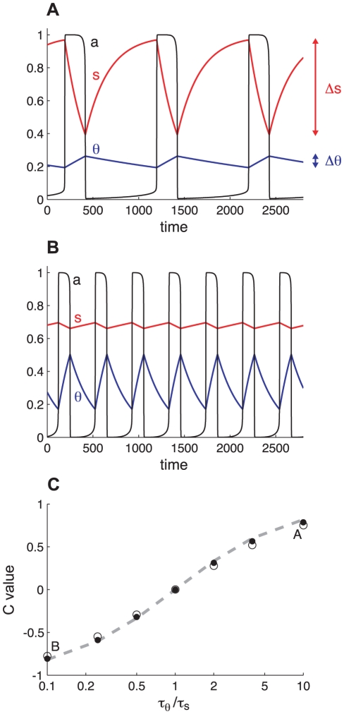
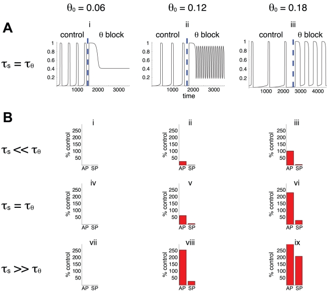
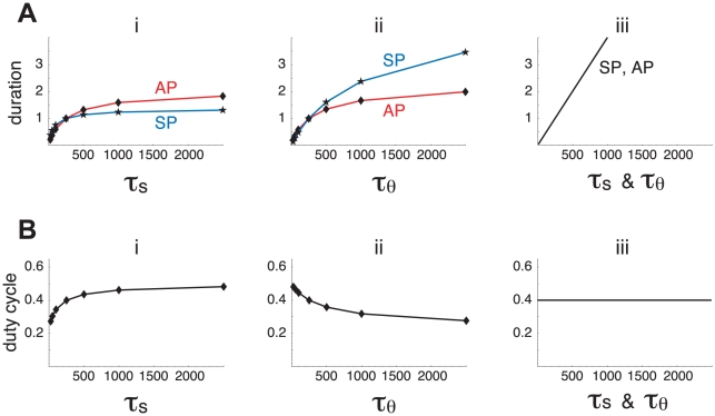
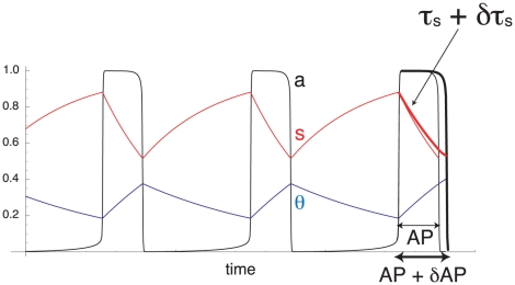
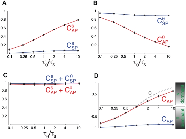
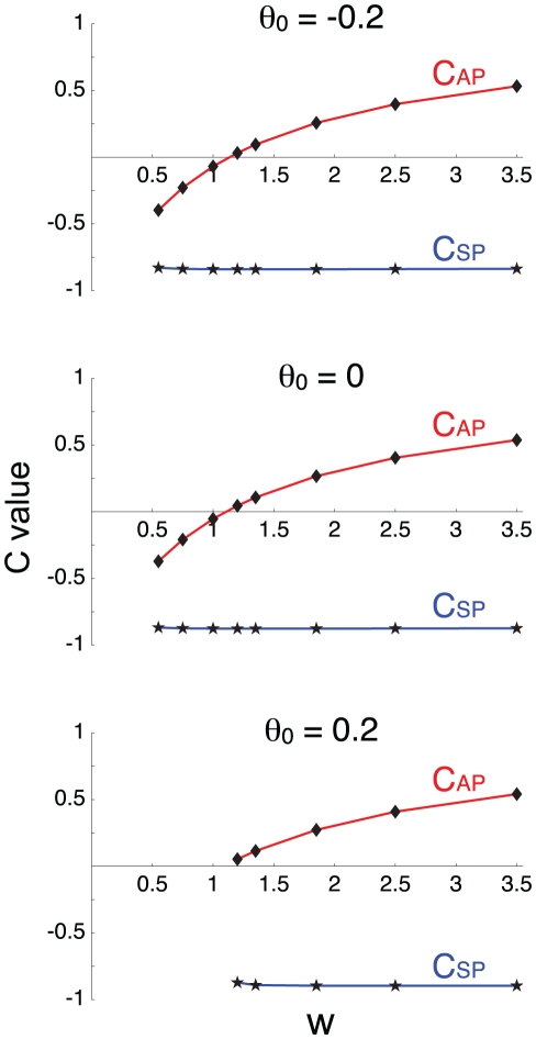
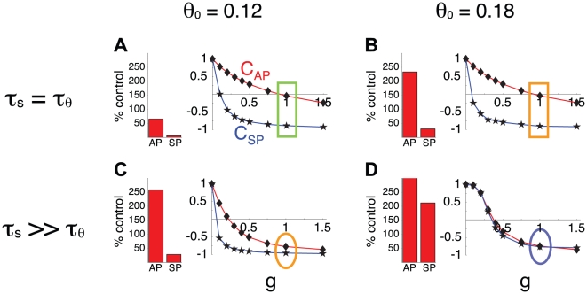
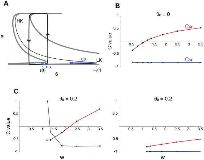
Biological systems are characterized by a high number of interacting components. Determining the role of each component is difficult, addressed here in the context of biological oscillations. Rhythmic behavior can result from the interplay of positive feedback that promotes bistability between high and low activity, and slow negative feedback that switches the system between the high and low activity states. Many biological oscillators include two types of negative feedback processes: divisive (decreases the gain of the positive feedback loop) and subtractive (increases the input threshold) that both contribute to slowly move the system between the high- and low-activity states. Can we determine the relative contribution of each type of negative feedback process to the rhythmic activity? Does one dominate? Do they control the active and silent phase equally? To answer these questions we use a neural network model with excitatory coupling, regulated by synaptic depression (divisive) and cellular adaptation (subtractive feedback). We first attempt to apply standard experimental methodologies: either passive observation to correlate the variations of a variable of interest to system behavior, or deletion of a component to establish whether a component is critical for the system. We find that these two strategies can lead to contradictory conclusions, and at best their interpretive power is limited. We instead develop a computational measure of the contribution of a process, by evaluating the sensitivity of the active (high activity) and silent (low activity) phase durations to the time constant of the process. The measure shows that both processes control the active phase, in proportion to their speed and relative weight. However, only the subtractive process plays a major role in setting the duration of the silent phase. This computational method can be used to analyze the role of negative feedback processes in a wide range of biological rhythms.

Figure 1. Illustration of the concept that the faster process contributes more to rhythm generation.

A. Time courses of activity (a, black), the synaptic recovery variable (s, red), and the adaptation variable (θ, blue) for τ_θ/τ_s = 10. The range of variation of s (Δs) is about 10 times larger than the range of variation of θ (Δθ). Thus, according to the correlative measure s contributes more to the rhythmicity. B. Similar time courses for τ_θ/τ_s = 0.1. The cellular adaptation now appears to contribute more than the synaptic recovery variable. C. Plot of the variations of C =  (R−1)/(R+1) with the τ_θ/τ_s ratio. Closed circles obtained from simulations with θ₀ = 0; open circles for θ₀ = 0.18. When θ is much faster than s (τ_θ/τ_s is small), C is close to -1 indicating that θ is the dominant process. When τ_θ ≈ τ_s, C≈0 indicating that both processes have equal contribution to the rhythm. At large τ_θ/τ_s, C approaches 1 and s is the dominant process. Points labeled A and B refer to the cases illustrated in panels A and B. Dashed curve, variations of c = (r−1)/(r+1) with τ_θ/τ_s; r = (w/g)(τ_θ/τ_s) and w = g = 1. Results are similar if we keep τ_θ/τ_s = 1 and vary w/g instead.

Figure 2. Illustration of the blockade approach.

A. time course of network activity before (“control,” g = 1) and after (“θ block,” g = 0) blocking the adaptation process θ. These simulations were obtained for τ_θ/τ_s = 1 and for the three values of θ₀ indicated. Vertical dashed line indicates the time when the process was blocked. B. Effects of blocking θ on the lengths of the active and silent phases (AP, SP), represented as percentage of “control”. No bars are shown when rhythmic activity was abolished. There are more cases where θ block results in decrease of SP duration (ii, iii, v, vi, viii) than increase in AP duration (vi, viii, ix). The interpretation is that θ contributes more to delay episode onset than to provoke episode termination. The results of the blockade experiment depend on the value of θ₀, the activity threshold in the absence of adaptation, unlike the predictions from the correlative approach (Figure 1C). The blockade experiments also produces similar results in pairs of cases (iii, v) and (vi, viii) that have different τ_θ/τ_s ratio; this is also in opposition to the correlative approach.

Figure 3. Variations of the time constants τ_s and τ_θ have different effects on the activity pattern.

A. Relative change in AP (red, diamonds) and SP (blue, stars) as τ_s (i) or τ_θ (ii) is varied. For comparison, the linear change in both AP and SP when τ_θ and τ_s are varied together by the same factor is shown (iii, τ_s & τ_θ). B. Variations of the duty cycle with τ_s (i), τ_θ (ii) and τ_s & τ_θ (iii).

Figure 4. Construction of a measure of the contribution of s to episode termination.

Increasing τ_s by δτ_s at the beginning of an episode slows down s slightly (thick red curve), so the active phase is lengthened by δAP (thick black curve).

Figure 5. Variations of the contributions of s and θ with τ_θ/τ_s.

A. Contributions of s to episode termination (C^s _AP, red, diamonds) and initiation (C^s _SP, blue, stars). B. Contributions of θ to episode termination (C^θ _AP, red, diamonds) and initiation (C^θ _SP, blue, stars). C. Both sums C^s _AP + C^θ _AP (red, diamonds) and C^s _SP + C^θ _SP (blue, stars) are close to 1, demonstrating the consistency of the measures. D. Combined measures C_AP (red, diamonds) and C_SP (blue, stars), as defined in Eq 11–12, superimposed with the prediction from the correlative measure c (dashed curve, as in Figure 1C). C_AP≈−1: θ controls the active phase; C_AP≈0: both θ and s have equal contributions to setting the duration of the active phase; C_AP≈1: s controls the active phase (and similarly for C_SP and the silent phase). Variations of C_AP show that the relative contribution of s to the termination of the active phase increases with τ_θ/τ_s, in agreement with the correlative approach. On the other hand, C_SP remains close to -1, showing that the subtractive process (θ) controls episode onset over the whole range.

Figure 6. Variations of C_AP and C_SP with network connectivity and cell excitability (for τ_θ/τ_s = 1, g = 1).

C_AP increases with increased synaptic connectivity, as would be expected from the correlative measure (Eq 4), with equal contributions from both processes (C_AP = 0) when (w/g) (τ_θ/τ_s)  = 1. In contrast, C_SP is always close to -1, the subtractive feedback process sets the length of the silent phase regardless of the value of w. Finally, both C_AP and C_SP are unaffected by changes in θ₀, showing that cell excitability does not influence which process controls episodic activity.

Figure 7. The blockade experiment does not inform on the relative contributions of each process to rhythmic activity.

Panels A, B, C, D correspond to cases shown in panels v, vi, viii, ix in Figure 2. For each case, the change in AP and SP durations following θ block is shown next to the variations of C_AP (red, diamonds) and C_SP (blue, stars) with g (the maximum amplitude of cellular adaptation). Blocking θ means changing g from 1 to 0. As g reaches 0, both C_AP and C_SP reach 1 since s becomes the only variable controlling episodic activity. In A and B, the contributions measures are also the same before the block (g = 1, rectangle highlights), nevertheless the blockade leads to different changes in AP and SP durations. Thus, these changes in durations after the block cannot be used to predict the respective contributions of each process before the block. Panels C and D illustrate the same points, with similar contributions measures before the block (oval highlights) but different effects of the block on AP and SP durations. Finally, panels B and C show that despite different contributions measures (oval vs. rectangle highlight) before the block, the resulting effect of the block on AP and SP durations are the same. Again, results from the block do not provide much information about the respective contributions of each process before the block.

Figure 8. Alternate estimation of the relative contributions of each process using phase plane analysis.

A. Representation of the system in the a,s-plane. The system trajectory is shown as a thick black curve with arrows at the transitions between activity phases. The trajectory follows the dynamic nullcline (thin black S-shaped curve) which moves left during the silent phase and reaches the thick gray nullcline on the left at episode onset. At onset, the trajectory reaches the low knee (s(t) = s _k(t)). During the active phase, the dynamic nullcline moves to the right toward the thick gray nullcline on the right. It reaches it at episode termination, as the trajectory reaches the high knee. Note that the lower portion of the nullcline is much more sensitive to θ than the higher portion. LK, low knee; HK, high knee of the a-nullcline. B. Variations of C_AP and C_SP (calculated using the phase plane approximation illustrated in A) with w (for τ_θ/τ_s = 1 and θ₀ = 0). There is good agreement with the computational method based on small perturbations in the time constants (compare with Figure 6B). C. For large values of θ₀, such that high activity episodes require that θ be close to 0, the computational calculation of the relative contributions (left panel) and the phase plane estimation (right panel) can disagree. In the case shown, τ_θ/τ_s = 0.1 (w = g = 1), so the phase plane method estimates that θ should control both active and silent phase (right panel). The disagreement with the computed C_AP and C_SP (left panel) is a result of the geometric argument used to estimate the contributions neglecting the fact that the speed of variation of s and θ can slow down dramatically when approaching their asymptotic values (see text).

References

1. Tsai TY, Choi YS, Ma W, Pomerening JR, Tang C, et al. Robust, tunable biological oscillations from interlinked positive and negative feedback loops. Science. 2008;321:126–129. - PMC - PubMed
1. Tyson JJ. Modeling the cell division cycle: cdc2 and cyclin interactions. Proc Natl Acad Sci U S A. 1991;88:7328–7332. - PMC - PubMed
1. van der Pol B, van der Mark J. The heartbeat considered as a relaxation oscillation, and an electrical model of the heart. Phil Mag. 1928;6:763–775.
1. Rinzel J, Ermentrout B. Analysis of neural excitability and oscillations. In: Koch C, Segev I, editors. Methods in Neuronal Modeling: From Synapses to Networks. Cambridge, MA: MIT Press; 1989.
1. Kurosawa G, Aihara K, Iwasa Y. A model for the circadian rhythm of cyanobacteria that maintains oscillation without gene expression. Biophys J. 2006;91:2015–2023. - PMC - PubMed
Publication types