Robust statistical label fusion through COnsensus Level, Labeler Accuracy, and Truth Estimation (COLLATE)

Abstract

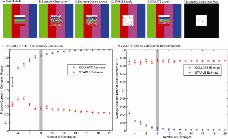
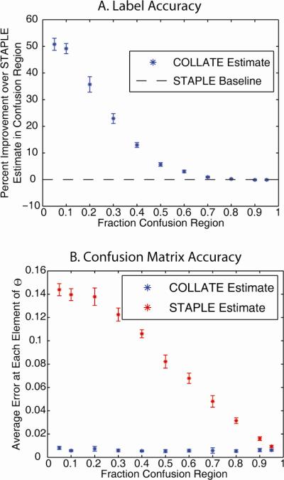
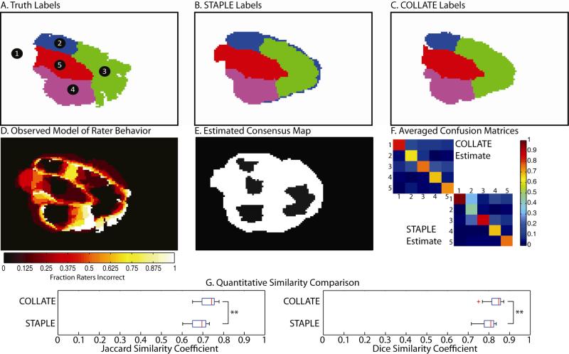
Segmentation and delineation of structures of interest in medical images is paramount to quantifying and characterizing structural, morphological, and functional correlations with clinically relevant conditions. The established gold standard for performing segmentation has been manual voxel-by-voxel labeling by a neuroanatomist expert. This process can be extremely time consuming, resource intensive and fraught with high inter-observer variability. Hence, studies involving characterizations of novel structures or appearances have been limited in scope (numbers of subjects), scale (extent of regions assessed), and statistical power. Statistical methods to fuse data sets from several different sources (e.g., multiple human observers) have been proposed to simultaneously estimate both rater performance and the ground truth labels. However, with empirical datasets, statistical fusion has been observed to result in visually inconsistent findings. So, despite the ease and elegance of a statistical approach, single observers and/or direct voting are often used in practice. Hence, rater performance is not systematically quantified and exploited during label estimation. To date, statistical fusion methods have relied on characterizations of rater performance that do not intrinsically include spatially varying models of rater performance. Herein, we present a novel, robust statistical label fusion algorithm to estimate and account for spatially varying performance. This algorithm, COnsensus Level, Labeler Accuracy and Truth Estimation (COLLATE), is based on the simple idea that some regions of an image are difficult to label (e.g., confusion regions: boundaries or low contrast areas) while other regions are intrinsically obvious (e.g., consensus regions: centers of large regions or high contrast edges). Unlike its predecessors, COLLATE estimates the consensus level of each voxel and estimates differing models of observer behavior in each region. We show that COLLATE provides significant improvement in label accuracy and rater assessment over previous fusion methods in both simulated and empirical datasets.

Fig. 1

The inaccuracies of the STAPLE model of rater behavior. A representative slice from the truth model is shown in (A). The expected STAPLE model of rater behavior can be seen in (B). STAPLE operates under the assumption that there is a uniform probability that any given rater would mis-label a given voxel. The observed model of rater behavior can be seen in (C). The primary difference between (B) and (C) is that the human raters showed a clear inclination to mislabel boundary pixels and other ambiguous regions.

Fig. 2

The COLLATE model. The hidden data in the COLLATE E-M algorithm can be seen in (A), (B) and (C). These images (the true labels, rater confusion matrices and consensus map) represent the complete set of data that COLLATE attempts to estimate. The generative model of rater behavior can be seen in (D). This flowchart shows the path from an input voxel on some clinical data to a single observation. A flowchart demonstrating the way in which COLLATE takes input observations and estimates the hidden data can be seen in (E). Note the inclusion of priors in conditional probability that is estimated to generate the maximum a posteriori estimate of the hidden data. Example estimates of the hidden data can be seen in (F), (G) and (H). These images are meant for visual inspection and demonstration of the COLLATE algorithm.

Fig 3

Results for simulation 1 using the COLLATE model of rater behavior. A representative slice from the truth model can be seen in (A). (B) and (C) represent example observations of the slice seen in (A). The STAPLE estimate using 8 coverages can be seen in (D). The COLLATE estimate using the same observations can be seen in (E). Note the improvement of the estimate seen in (E) over the estimate seen in (D). The estimated consensus map can be seen in (F). These are the expected results given the behavior of the raters seen in (B) and (C). The truth estimation accuracy comparison of the two algorithms in the confusion region for varying numbers of coverages can be seen in (G). The confusion matrix accuracy comparison for varying number of coverages can be seen in (H). The gray bars seen on (G) and (H) correspond to the number of coverages used in the estimations seen in (D), (E) and (F).

Fig 4

Results for simulation 2, the COLLATE sensitivity with respect to the estimated confusion region size data-adaptive prior. The sensitivity of the confusion region size prior can be seen in (A) and (B). (A) represents the accuracy of the truth estimation with varying prior estimates from 0.05 to 0.95 for a given confusion region size of 0.5. The accuracy of the truth estimation is presented as a percent improvement over the STAPLE estimate for the same set of input observations. (B) represents the accuracy of the confusion matrix estimation with varying prior estimates from 0.05 to 0.95 for a given confusion region size of 0.5. All data presented in this Figure use six coverages for both COLLATE and STAPLE.

Fig 5

Results for simulation 2, the accuracy of the COLLATE algorithm with respect to the confusion region size. This tests the ability of the algorithm to estimate the confusion region size. (A) represents the percent improvement for COLLATE over the STAPLE estimation for confusion region sizes varying from 0.05 to 0.95. (B) represents the average absolute error at each element in the confusion matrices for varying confusion region size. Note that the COLLATE estimate accuracy remains constant while the quality of the STAPLE estimate varies depending upon the size of the confusion region. All data presented in this Figure use six coverages for both COLLATE and STAPLE.

Fig 6

Results for simulation 3 using boundary random raters. A representative slice from the truth model can be seen in (A). The numbers on (A) identify the numbers corresponding with the given labels so that the confusion matrix representations can be fully understood. (B) and (C) represent example observations of the slice seen in (A). The STAPLE estimate using eight coverages can be seen in (D). The COLLATE estimate using the same observations can be seen in (E). Note the improvement of the estimate seen in (E) over the estimate seen in (D). The estimated consensus map can be seen in (F). These are the expected results given the behavior of the raters seen in (B) and (C). The truth estimation accuracy comparison of the two algorithms in the confusion region for varying numbers of coverages can be seen in (G). The gray bar indicates the number of coverages corresponding to the estimates seen in (D), (E). (F), (H) and (I). An example confusion matrix from a single rater from the STAPLE estimate and the COLLATE estimate using eight coverages can be seen in (H) and (I), respectively.

Fig 7

Empirical experiment using human raters. A representative slice from the 10-slice truth model can be seen in (A). The numbers on (A) identify the numbers corresponding with the given labels so that the confusion matrix representations can be fully understood. The STAPLE estimate using eight coverages can be seen in (B). The COLLATE estimate using the same observations can be seen in (C). Note the improvement of the estimate seen in (C) over the estimate seen in (B). The observed model of rater behavior can be seen in (D). The color value at each voxel corresponds to the fraction of raters that incorrectly labeled the given voxel. The estimated consensus map can be seen in (E). This is a rather conservative estimate, but it is the expected result given that P(C=0) = 0.99. The averaged confusion matrices for both the STAPLE and COLLATE estimations can be seen in (F). Note the fact that the COLLATE estimate appears to be a nearly constant valued diagonal matrix, while the STAPLE estimate is biased towards certain labels, particularly the background (first column). The range of Jaccard Similarity Coefficient values and Dice Similarity Coefficient values can be seen in (G). In both cases, a paired t-test results in a p-value of less that 0.001, indicating that the COLLATE estimates are significantly better than the STAPLE estimates.

Fig 8

Results for simulation 4 using STAPLE model of rater behavior. A representative slice from the truth model can be seen in (A). (B) and (C) represent example observations of the slice seen in (A). The STAPLE estimate using eight coverages can be seen in (D). The COLLATE estimate using the same observations can be seen in (E). The estimated consensus map can be seen in (F). The true consensus map would indicate that the entire map is a confusion region, but due to the fact that some raters agree at various voxels, consensus is estimated at isolated voxels. The truth estimation accuracy comparison of the two algorithms for varying numbers of coverages can be seen in (G). The mean COLLATE estimate is slightly better for low numbers of coverages, but both COLLATE and STAPLE converge to the same accuracy level for seven or more coverages. The confusion matrix accuracy comparison for varying number of coverages can be seen in (H). The gray bars seen on (G) and (H) correspond to the number of coverages used in the estimations seen in (D), (E) and (F).

References

1. Warfield S, et al. Automatic identification of gray matter structures from MRI to improve the segmentation of white matter lesions. J Image Guid Surg. 1995;1:326–38. - PubMed
1. Kikinis R, et al. Routine quantitative analysis of brain and cerebrospinal fluid spaces with MR imaging. J Magn Reson Imaging. 1992 Nov-Dec;2:619–29. - PubMed
1. Ho TK, et al. Decision Combination in Multiple Classifier Systems. IEEE Transactions on Pattern Analysis and Machine Intelligence. 1994 Jan;16:66–75.
1. Kittler J, et al. On combining classifiers. IEEE Transactions on Pattern Analysis and Machine Intelligence. 1998 Mar;20:226–239.
1. Windridge D, Kittler J. A morphologically optimal strategy for classifier combination: Multiple expert fusion as a tomographic process. IEEE Transactions on Pattern Analysis and Machine Intelligence. 2003 Mar;25:343–353.
Publication types