. 2011 Dec 22;278(1725):3723-30.
doi: 10.1098/rspb.2011.0435. Epub 2011 May 4.

A dimensionless number for understanding the evolutionary dynamics of antigenically variable RNA viruses

Affiliations

A dimensionless number for understanding the evolutionary dynamics of antigenically variable RNA viruses

Katia Koelle et al. Proc Biol Sci. .

Abstract

Antigenically variable RNA viruses are significant contributors to the burden of infectious disease worldwide. One reason for their ubiquity is their ability to escape herd immunity through rapid antigenic evolution and thereby to reinfect previously infected hosts. However, the ways in which these viruses evolve antigenically are highly diverse. Some have only limited diversity in the long-run, with every emergence of a new antigenic variant coupled with a replacement of the older variant. Other viruses rapidly accumulate antigenic diversity over time. Others still exhibit dynamics that can be considered evolutionary intermediates between these two extremes. Here, we present a theoretical framework that aims to understand these differences in evolutionary patterns by considering a virus's epidemiological dynamics in a given host population. Our framework, based on a dimensionless number, probabilistically anticipates patterns of viral antigenic diversification and thereby quantifies a virus's evolutionary potential. It is therefore similar in spirit to the basic reproduction number, the well-known dimensionless number which quantifies a pathogen's reproductive potential. We further outline how our theoretical framework can be applied to empirical viral systems, using influenza A/H3N2 as a case study. We end with predictions of our framework and work that remains to be done to further integrate viral evolutionary dynamics with disease ecology.


Figures

Figure 1.
Figure 1.
Phylogenetic trees of several antigenically variable RNA viruses. (a) Influenza A/H3N2's HA phylogeny in humans, inferred from sequences isolated between 1968 and 2003. (b) HIV's gp120 phylogeny (C2-V5 region), inferred from sequences isolated in the US between 1981 and 2007. (c) Influenza B's HA phylogeny, inferred from sequences isolated between 1973 and 2008. In all subplots, concentric circles measure time.
Figure 2.
Figure 2.
A comparison between the analytical expressions used to calculate κ and stochastic simulations of the simplified epidemiological model. (a) A representative simulation showing the dynamics of variant X (bold black) and variant Y (grey), alongside the analytical expression for IX(t) (black), given by equation (2.8). (b) For the simulation shown in (a), the probability that a new variant, emerging at time t, successfully invades (u(t), bold black) alongside its assumed analytical value given by equation (2.9) (black). u(t) is calculated from the simulation as 1 − 1/(R0(S(t)/N)), where S(t) is the number of individuals susceptible, at time t, to an offspring variant that has not yet emerged. Simulation parameters are N = 18 million, R0 = 10, ν = 1/6 d−1, μ = 1/40 yr−1 and σ = 0.85. In both (a) and (b), the first vertical line shows the time of variant Y's emergence and the second vertical line shows the time of variant X's exclusion. (c) The distribution of times to the emergence of variant Y from 500 simulations of the simplified epidemiological model (bars), alongside the probability density function, gY(t). Simulation parameters are as in (a,b), with additional parameters kW = 1 and λW = 10 000. Vertical solid black line shows the mean of the 500 simulated times to emergence. Vertical dotted line shows the analytical expected time to emergence (equation (2.13)). (d) Same as in (c), only with kW = 3 and λW = 120. (eg) Distributions for the number of excess variants, from 100 simulations of the simplified epidemiological model (grey bars), alongside Poisson distributions with mean κ (black bars). In all three subplots, simulation parameters were N = 100 million, R0 = 10, ν = 1/10 d−1, μ = 1/70 yr−1, σ = 0.9 and λW = 2000. (e) Number of excess variants from 100 simulations, each with kW = 3.34, yielding κ = 0.05. The mean number of excess variants, computed from the simulation results, is 0.09. (f) Number of excess variants from 100 simulations, each with kW = 2.01, yielding κ = 0.15. The mean number of excess variants, computed from the simulation results, is 0.17. (g) Number of excess variants from 100 simulations, each with kW = 1.476, yielding κ = 0.50. The mean number of excess variants, computed from the simulation results, is 0.42. The number of excess variants for a given simulation was calculated by subtracting one from the number of variants co-circulating in the population 5 years after the extinction of variant X. We used a likelihood-ratio test to determine whether the null hypothesis (that the number of excess variants comes from a Poisson distribution with mean κ) could be rejected at the 95% confidence level in any of the three cases (eg) above. In none of the three cases could this null hypothesis be rejected.
Figure 3.
Figure 3.
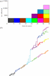
Long-term patterns of antigenic evolution and their dependence on κ. (a) A single stochastic realization of long-term antigenic evolution, given a κ value of 0.2, an equilibrium number of I = 3000 infected individuals and a generation time of 5 years. Different colours represent different antigenic variants. Over the first three generations, none of the endemic variants generate any excess variants. In the fourth generation, a single excess variant is generated. In the fifth generation, one of the two endemic variants generates no excess variants while the other generates one excess variant. In the sixth generation, two of the three endemic variants generate no excess variants while the third generates one excess variant. (b) A representative phylogeny arising from the diversification dynamics shown in (a). The phylogeny was constructed using a neutral coalescent model to generate the branching structure within clusters while the ancestral relationships among clusters and their emergence and death times were determined by the dynamics shown in (a). The topology represents one realization of the phylogenetic patterns possible under the given epidemiological dynamics. Colours of the branches correspond to the variant designations shown in (a).
Figure 4.
Figure 4.
Applying the κ framework to the empirical host–virus systems. (a) An antigenically-typed phylogeny that was simulated using the stochastic forward model described in §2b. The model was simulated for 16 generations using a κ value of 0.18. (b) Log-likelihood values for a range of κ values, calculated from the likelihood expression provided in the text. Solid vertical line indicates the true value of κ = 0.18, dotted line is the maximum-likelihood estimate of κ and the dashed lines are the 95% CI. (c) An antigenically-typed phylogeny of influenza A/H3N2 from sequences isolated between 1968 and 2003. Reproduced from Koelle et al. [13]. (d) Log-likelihood values for a range of κ values calculated from the distribution of excess variants deduced from the phylogeny in (c). (e) The duration of time each antigenic cluster persisted, defined as the amount of time between when a cluster emerges and when it generates its first successful offspring variant. The mean cluster persistence time is 3.51 years. Black curve shows the gY(t) for the best estimate of kW and λW, calculated as follows: I was first computed from estimates of the annual attack rate, N and ν, u was then computed using equation (2.9), given estimates of R0 and σ. Using these values of I and u, and for given values of kW and λW, the probability of observing each of the estimated cluster persistence times can be calculated using equation (2.12). The maximum-likelihood estimates of kW and λW were found by searching (kW and λW) parameter space for the maximum product of these probabilities, yielding kW = 2.26 and λW = 1162. (f) The probability of observing a given number of co-circulating antigenic variants in 2011. These probabilities were computed using equation (2.15), knowing that there was only one circulating variant in 2003 (FU02) and that a generation lasts approximately 3.5 years, and assuming that κ = 0.11.

Similar articles

Cited by

References

    1. Holmes E. C., Grenfell B. T. 2009. Discovering the phylodynamics of RNA viruses. PLoS Comput. Biol. 5, e1000505.10.1371/journal.pcbi.1000505 (doi:10.1371/journal.pcbi.1000505) - DOI - DOI - PMC - PubMed
    1. Rott N. 1990. Note on the history of the Reynolds number. Ann. Rev. Fluid Mech. 22, 1–1110.1146/annurev.fl.22.010190.000245 (doi:10.1146/annurev.fl.22.010190.000245) - DOI - DOI
    1. Anderson R. M., May R. M. 1991. Infectious diseases of humans: dynamics and control. Oxford, UK: Oxford University Press
    1. Grenfell B. T., Pybus O. G., Gog J. R., Wood J. L. N., Daly J. M., Mumford J. A., Holmes E. D. C. 2004. Unifying the epidemiological and evolutionary dynamics of pathogens. Science 303, 327–33210.1126/science.1090727 (doi:10.1126/science.1090727) - DOI - DOI - PubMed
    1. Andreasen V., Sasaki A. 2006. Shaping the phylogenetic tree of influenza by cross-immunity. Theoret. Popul. Biol. 70, 164–17310.1016/j.tpb.2006.04.004 (doi:10.1016/j.tpb.2006.04.004) - DOI - DOI - PubMed

Publication types

Substances