Using Blur to Affect Perceived Distance and Size

Abstract

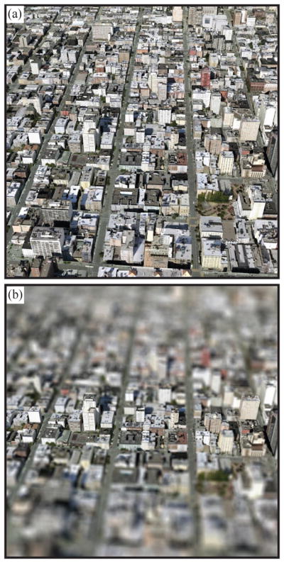
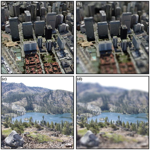
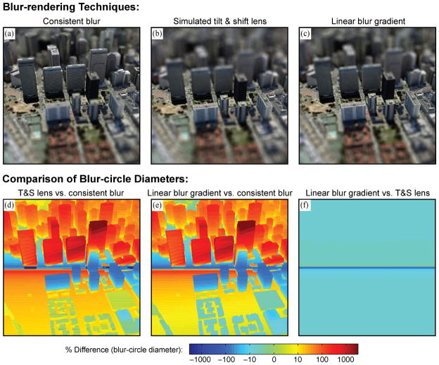
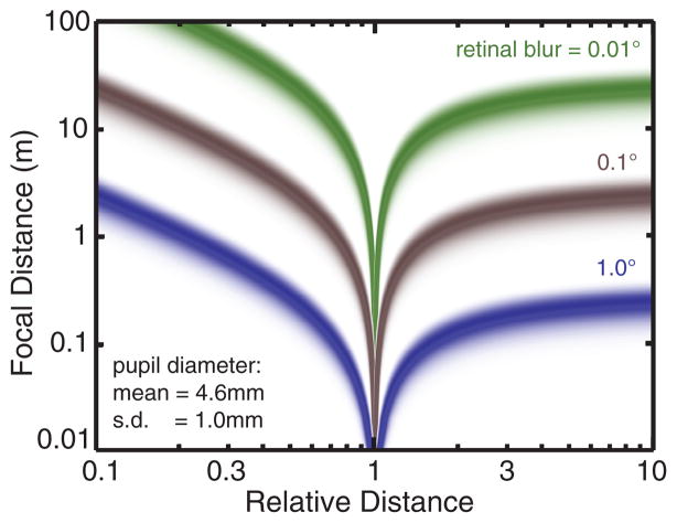
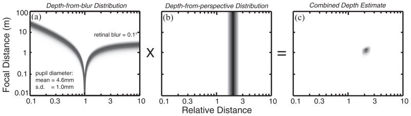
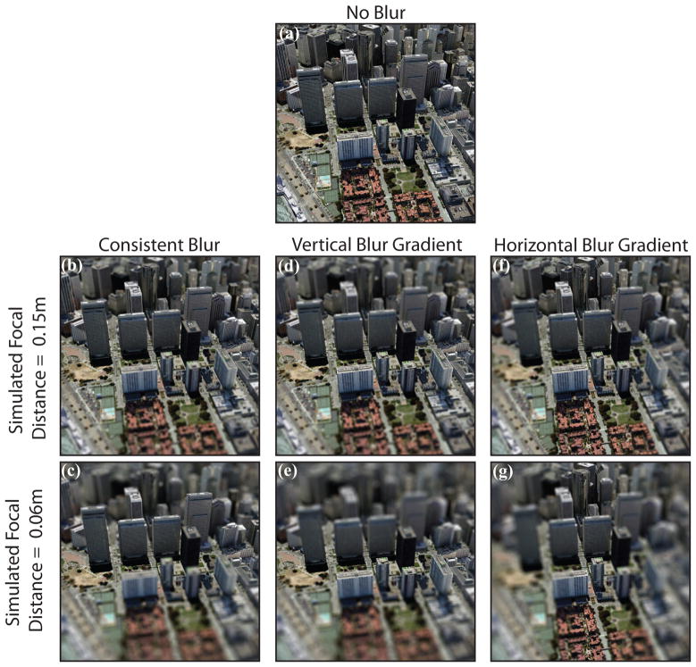
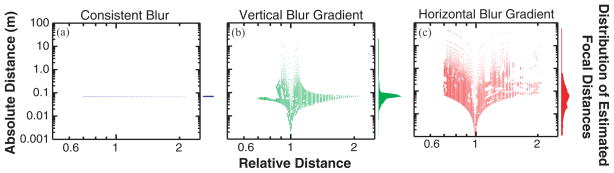
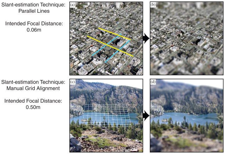
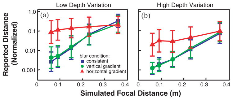
We present a probabilistic model of how viewers may use defocus blur in conjunction with other pictorial cues to estimate the absolute distances to objects in a scene. Our model explains how the pattern of blur in an image together with relative depth cues indicates the apparent scale of the image's contents. From the model, we develop a semiautomated algorithm that applies blur to a sharply rendered image and thereby changes the apparent distance and scale of the scene's contents. To examine the correspondence between the model/algorithm and actual viewer experience, we conducted an experiment with human viewers and compared their estimates of absolute distance to the model's predictions. We did this for images with geometrically correct blur due to defocus and for images with commonly used approximations to the correct blur. The agreement between the experimental data and model predictions was excellent. The model predicts that some approximations should work well and that others should not. Human viewers responded to the various types of blur in much the way the model predicts. The model and algorithm allow one to manipulate blur precisely and to achieve the desired perceived scale efficiently.

Fig. 1

(a) Rendering a cityscape with a pinhole aperture results in no perceptible blur. The scene looks large and far away. (b) Simulating a 60m-wide aperture produces blur consistent with a shallow depth of field, making the scene appear to be a miniature model. Original city images and data from GoogleEarth are copyright Terrametrics, SanBorn, and Google.

Fig. 2

Upper two images: Another example of how rendering an image with a shallow depth of field can make a downtown cityscape appear to be a miniature-scale model. The left image was rendered with a pinhole camera, the right with a 60m aperture. Lower two images: Applying a blur gradient that approximates a shallow depth of field can also induce the miniaturization effect. The effects are most convincing when the images are large and viewed from a short distance. Original city images and data from GoogleEarth are copyright Terrametrics, SanBorn, and Google. Original lake photograph is copyright Casey Held.

Fig. 3

Schematic of blur in a simple imaging system. z₀ is the focal distance of the device given the lens focal length, f, and the distance from thelens to the image plane, s₀. An object at distance z₁ creates a blur circle of diameter c₁, given the device aperture, A. Objects within the focal plane will be imaged in sharp focus. Objects off the focal plane will be blurred proportional to their dioptric (m⁻¹) distance from the focal plane.

Fig. 4

The Scheimpflug principle. Tilt-and-shift lenses cause the orientation of the focal plane to shift and rotate relative to the image plane. As a result, the apparent depth of field in an image can be drastically changed and the photographer has greater control over which objects are in focus and which are blurred.

Fig. 5

Comparison of blur patterns produced by three rendering techniques: consistent blur (a), simulated tilt-and-shift lens (b), and linear blur gradient (c). The settings in (b) and (c) were chosen to equate the maximum blur-circle diameters with those in (a). The percent differences in blur-circle diameters between the images are plotted in (d), (e), and (f). Panels (d) and (e) show that the simulated tilt-and-shift lens and linear blur gradient do not closely approximate consistent blur rendering. The large differences are due to the buildings, which protrude from the ground plane. Panel (f) shows that the linear blur gradient provides essentially the same blur pattern as a simulated tilt-and-shift lens. Most of the differences in (f) are less than 7%; the only exceptions are in the band near the center, where the blur diameters are less than one pixel and not detectable in the final images.

Fig. 6

Focal distance as a function of relative distance and retinal-image blur. Relative distance is defined as the ratio of the distance to an object and the distance to the focal plane. The three colored curves represent different amounts of image blur expressed as the diameter of the blur circle, c, in degrees. We use angular units because in these units, the image device’s focal length drops out [Kingslake 1992]. The variance in the distribution was determined by assuming that pupil diameter is Gaussian distributed with a mean of 4.6mm and standard deviation of 1mm [Spring and Stiles 1948]. For a given amount of blur, it is impossible to recover the original focal distance without knowing the relative distance. Note that as the relative distance approaches 1, the object moves closer to the focal plane. There is a singularity at a relative distance of 1 because the object is by definition completely in focus at this distance.

Fig. 7

Bayesian analysis of blur as cue to absolute distance. (a) The probability distribution P(z_o, d|c) where c is the observed blur diameter in the image (in this case, 0.1°), z₀ is the focal distance, and d is the relative distance of another point in the scene. Measuring the blur produced by an object cannot reveal the absolute or relative distance to points in the scene. (b) The probability distribution P(z_o, d|p) where p is the observed perspective. Perspective specifies the relative distance, but not the absolute distance: it is scale ambiguous. (c) The product of the distributions in (a) and (b). From this posterior distribution, the absolute and relative distances of points in the scene can be estimated.

Fig. 8

The four types of blur used in the analysis and experiment: (a) no blur, (b) and (c) consistent blur, (d) and (e) linear vertical blur gradient, and (f) and (g) linear horizontal blur gradient. Simulated focal distances of 0.15m (b,d,f) and 0.06m (c,e,g) are shown. In approximating the blur produced by a short focal length, the consistent-blur condition produces the most accurate blur, followed by the vertical gradient, the horizontal gradient, and the no-blur condition. Original city images and data from GoogleEarth are copyright Terrametrics, SanBorn, and Google.

Fig. 9

Determining the most likely focal distance from blur and perspective. Intended focal distance was 0.06m. Each panel plots estimated focal distance as a function of relative distance. The left, middle, and right panels show the estimates for consistent blur, vertical blur gradient, and horizontal blur gradient, respectively. The first step in the analysis is to extract the relative-distance and blur information from several points in the image. The values for each point are then used with Eq. (2) to estimate the focal distance. Each estimate is represented by a point. Then all of the focal distance estimates are accumulated to form a marginal distribution of estimates (shown on the right of each panel). The data from a consistent-blur rendering most closely matches the selected curve, resulting in extremely low variance. Though the vertical blur gradient incorrectly blurs several pixels, it is well correlated with the relative distances in the scene, so it too produces a marginal distribution with low variance. The blur applied by the horizontal gradient is mostly uncorrelated with relative distance, resulting in a marginal distribution with large variance and therefore the least reliable estimate.

Fig. 10

Schematic of variables pertinent to the semiautomated blurring algorithm. Here, the image surface is equivalent to the monitor surface, and v and l are in units of pixels. σ indicates the angle between the ground plane’s surface normal and the imaging system’s optical axis. Refer to Algorithm 1 for details on how each value can be calculated from an input image. (Adapted from Okatani and Deguchi [2007].)

Fig. 11

Input and output of the semiautomated blurring algorithm. The algorithm can estimate the blur pattern required to simulate a desired focal length. It can either derive scene information from parallel lines in a scene or use manual feedback from the user on the overall orientation of the scene. (a) Two pairs of parallel lines were selected from a carpentered scene for use with the first approach. (b) The resulting image once blur was applied. Intended focal distance = 0.06m. (c) A grid was manually aligned to lie parallel to the overall scene. (d) The blurred output designed to simulate a focal distance of 0.50m.

Fig. 12

Results of the psychophysical experiment averaged across the seven subjects. Panels (a) and (b) respectively show the data when the images had low and high depth variation. The type of blur manipulation is indicated by the colors and shapes of the data points. Blue squares for consistent blur, green circles for vertical blur gradient, and red triangles for horizontal blur gradient. Error bars represent standard errors. Individual subject data are included in the supplemental material.

References

1. Akeley K, Watt SJ, Girshick AR, Banks MS. A stereo display prototype with multiple focal distances. ACM Trans Graph. 2004;23(3):804–813.
1. Barsky BA. Vision-Realistic rendering: Simulation of the scanned foveal image from wavefront data of human subjects. Proceedings of the 1st Symposium on Applied Perception in Graphics and Visualization (APGV’04); 2004. pp. 73–81.
1. Barsky BA, Horn DR, Klein SA, Pang JA, Yu M. Camera models and optical systems used in computer graphics: Part I, Object-Based techniques. Proceedings of the International Conference on Computational Science and its Applications (ICCSA’03), Montreal, 2nd International Workshop on Computer Graphics and Geometric Modeling (CGGM’03); 2003a. pp. 246–255.
1. Barsky BA, Horn DR, Klein SA, Pang JA, Yu M. Camera models and optical systems used in computer graphics: Part II, Image-Based techniques. Proceedings of the International Conference on Computational Science and its Applications (ICCSA’03), 2nd International Workshop on Computer Graphics and Geometric Modeling (CGGM’03); 2003b. pp. 256–265.
1. Bell JA. Theory of mechanical miniatures in cinematography. Trans SMPTE. 1924;18:119.