How should prey animals respond to uncertain threats?

Abstract

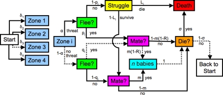
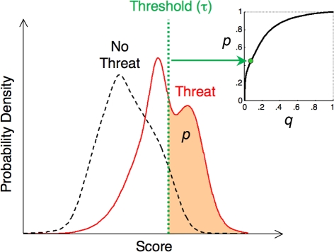
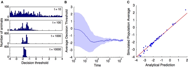
A prey animal surveying its environment must decide whether there is a dangerous predator present or not. If there is, it may flee. Flight has an associated cost, so the animal should not flee if there is no danger. However, the prey animal cannot know the state of its environment with certainty, and is thus bound to make some errors. We formulate a probabilistic automaton model of a prey animal's life and use it to compute the optimal escape decision strategy, subject to the animal's uncertainty. The uncertainty is a major factor in determining the decision strategy: only in the presence of uncertainty do economic factors (like mating opportunities lost due to flight) influence the decision. We performed computer simulations and found that in silico populations of animals subject to predation evolve to display the strategies predicted by our model, confirming our choice of objective function for our analytic calculations. To the best of our knowledge, this is the first theoretical study of escape decisions to incorporate the effects of uncertainty, and to demonstrate the correctness of the objective function used in the model.

Keywords: agent-based modeling; constrained optimization; decision making; escape decision; evolution; probabilistic automata; uncertainty.

Figure 1

Probabilistic automaton model of the life cycle of a prey animal. At each time step, every animal begins in the state “start,” and follows a complete path, ending either back at the start, or in death. Each arrow is labeled with the conditional probability that the given event occurs (die, survive, etc.), once the animal reaches the box at the tail of that arrow. The animal spots a potential threat in zone i with probability δ_i. Four zones (groupings by predator–prey distance) are shown in the diagram. The threat is real with probability α. If there is a threat the prey animal flees with probability p_i. Those animals that do not flee are killed with probability L_i, while those that do flee always escape. The animals that neither flee nor die mate with probability m, producing n progeny. The animals that do flee suffer a reduced mating rate of m(1 − R). In order to keep the population stable, some randomly selected animals are killed at the end of the time step with probability σ. The probability of any path is obtained by multiplying the conditional probabilities of each subsequent step. A sample path is illustrated by the dashed arrows in the diagram: The animal spots a potential threat in zone 3. This is not a real threat, but, with its imperfect information, the animal incorrectly decides to flee. It then mates, producing n progeny, which are added to the population for the next time step. The animal does not succumb to disease, starvation, or other non-predation-related causes of death, and lives on to the next time step. The probability of this path is δ₃(1 − α)q_im(1 − R)(1 − σ).

Figure 2

Connection between ROC curves (p vs. q) and probability distributions. The probability distributions of some “score” parameter, conditioned on the presence (solid curve) or absence (dashed curve) of a threat are shown. A possible interpretation for this score is that it is the output of a neural network that assesses all of the information available to the animal, in an attempt to infer the danger of a given object. One possible decision threshold, τ, is indicated, whereby the animal decides to flee from objects with scores above the threshold, and not to flee from those with scores below the threshold. By varying the threshold, the animal can alter the correct detection probability p, indicated by the area under the “threat” distribution (solid curve) to the right of the threshold; at the same time, varying the threshold also affects the false positive probability q, given by the area under the “no threat” distribution (dashed curve) to the right of the threshold. The same threshold determines both p and q; they are related by the ROC curve p = f(q) (inset).

Figure 3

The importance of economic factors in decision making increases with rising uncertainty about the environment. The departure of the optimal decision threshold (τ) from a MLE (described by τ = ω/2) is shown as a function of ω, the displacement between the means of the score distributions for threats and non-threats. The result is shown for several different values of f′(q), which contains all the economic factors, and quantifies how bold (large values) or timid (small values) the strategy is (see text). For large |ω|, threats are easily identified, and the strategies all converge to a maximum likelihood decision strategy: flee if and only if danger is more likely than not. As the uncertainty increases (small |ω|), the strategies diverge in a manner dictated by the economic factors.

Figure 4

Computer simulation confirms that our objective function, r = N^−1dN/dt, is indeed maximized by selection pressure. (A), Time evolution of the distribution of escape response thresholds across a population of simulated prey animals. The time (in units of time steps) at which the histogram was measured is indicated on each histogram. The population was initialized at time t = 0 with a uniform distribution of escape strategies. The model parameters for this simulation were (α,L,m,n,R,ω) = (0.15,0.8,0.02,4,0.5,−2.0), and the threshold of each progeny was equal to that of its parent, plus Gaussian noise with mean 0 and SD 0.01. (B), Average escape threshold across this simulated population asymptotes to the predicted value. The shaded region extends one SD above and below the average. At the end of this simulation, the population mean is −1.605 with SD 0.08, in good agreement with the theoretical value (Eq. 8) of −1.645. (C), Repeating this simulation 50 times with randomly selected parameter values shows good agreement between the analytical prediction and simulation results across the full range of parameter values tested (Table 1). Population average thresholds (after 10⁴ time steps) are plotted against the analytical prediction. The red line represents equality between the prediction and simulation.

References

1. Adler J., Wung-Wai T. (1974). Decision-making in bacteria: chemotactic response of Escherichia coli to conflicting stimuli. Science 184, 12921294.10.1126/science.184.4143.1292 - DOI - PubMed
1. Apfelbach R., Blanchard C., Blanchard R., Hayes R., McGregor I. (2005). The effects of predator odors in mammalian prey species: a review of field and laboratory studies. Neurosci. Biobehav. Rev. 29, 1123–114410.1016/j.neubiorev.2005.05.005 - DOI - PubMed
1. Benton T., Evans M. (1998). Measuring mate choice using correlation: the effect of sampling behaviour. Behav. Ecol. Sociobiol. 44, 91–9810.1007/s002650050520 - DOI
1. Bialek W., Setayeshgar S. (2005). Physical limits to biochemical signaling. Proc. Natl. Acad. Sci. U.S.A. 102, 10040–1004510.1073/pnas.0504321102 - DOI - PMC - PubMed
1. Blumstein D. (2003). Flight-initiation distance in birds is dependent on intruder starting distance. J. Wildl. Manage. 64, 852–85710.2307/3802692 - DOI
LinkOut - more resources