. 2011 May;7(5):e1002041.
doi: 10.1371/journal.pcbi.1002041. Epub 2011 May 5.

Temporal encoding in a nervous system

Affiliations

Temporal encoding in a nervous system

Zane N Aldworth et al. PLoS Comput Biol. 2011 May.

Abstract

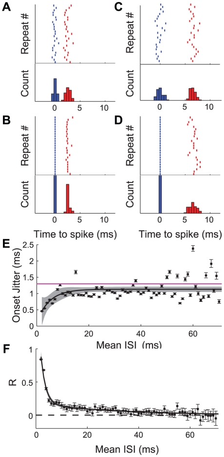
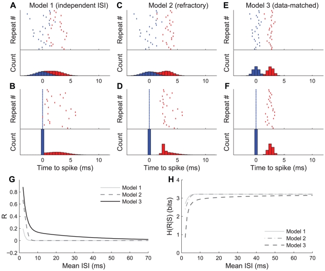
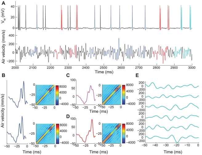
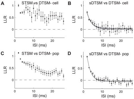
We examined the extent to which temporal encoding may be implemented by single neurons in the cercal sensory system of the house cricket Acheta domesticus. We found that these neurons exhibit a greater-than-expected coding capacity, due in part to an increased precision in brief patterns of action potentials. We developed linear and non-linear models for decoding the activity of these neurons. We found that the stimuli associated with short-interval patterns of spikes (ISIs of 8 ms or less) could be predicted better by second-order models as compared to linear models. Finally, we characterized the difference between these linear and second-order models in a low-dimensional subspace, and showed that modification of the linear models along only a few dimensions improved their predictive power to parity with the second order models. Together these results show that single neurons are capable of using temporal patterns of spikes as fundamental symbols in their neural code, and that they communicate specific stimulus distributions to subsequent neural structures.


Conflict of interest statement

The authors have declared that no competing interests exist.

Figures

Figure 1
Figure 1. Statistics of doublet spiking.
A: ±1 SD envelope showing intracellular voltage waveform relative to resting membrane potential of isolated single spikes (blue) and isolated short doublets of ISI 2.6 ms (red) from a single recording in interneuron of class 10-2a. Dashed black line denotes mean resting membrane potential (0 mV). B: ±1 SD of intracellular waveform from same recording as in A, this time with a doublet of ISI 6.5 ms (red, n = 26). C: ISI histogram of data from recording in A and B at 0.1 ms resolution (black line, n = 26,171 events), as well as compilation data from 40 cells of class 10-2a and 10-3a (gray shaded area, n = 577,435 events). D: Normalized ISI histogram of population data from panel C, with time scale reduced to 1–5 ms. Red line shows the recovery function, with black dashed line showing limits of fit to recovery function. E: Difference between independent model and measurements from data of joint probability of consecutive ISIs. Positive (red) values represent overestimation by the independent model, while negative (blue) values represent underpredictions by the independent model.
Figure 2
Figure 2. Spike-spike interactions in doublet patterns recorded in cricket interneurons.
A, Upper trace: A raster plot showing 25 of 85 responses to repeated presentations of a GWN stimulus, recording from the same cell as shown in Figure 1. The cell consistently responded to the stimulus by firing a doublet (first spike shown in blue, second spike in red) with average ISI of 2.6 ms. A, Lower trace: PSTH of all 85 responses from the raster, with the color convention conserved. B, upper and lower traces: Raster plot and PSTH showing same data from A, here aligned relative to the time of the first spike in the doublet (t = 0) rather than to the timing of the stimulus. This shows the variability in ISI across presentations of a single stimulus. C and D: Data from a second doublet event (mean ISI = 6.5 ms, 73 responses) from the same interneuron, data presentation conserved. E: jitter of arrival time of first spike in repeatable doublets recorded from 40 different cells in 32 animals, as a function of ISI (7753 events composed of 197,601 total pairs of spikes). Black line shows model fit to data (Eq. 1), with shaded area representing 95% confidence envelope around predictions from the model. Horizontal purple line shows population mean of single spike jitter from frozen noise method. F: estimate of correlation coefficient between first and second spikes in repeatable doublets (from same data set as in E). Error bars represent 95% confidence limits on estimation of correlation coefficient. Solid black line shows correlation coefficient as a function of ISI modeled as a double exponential (Eq. 2), with ±95% confidence interval on predictions from the model shown by the shaded grey region.
Figure 3
Figure 3. Three models of spike-spike interactions in doublet patterns.
A, Upper trace: raster plot of response from cell model 1 (independent ISI) to repeated presentations of a stimulus which reliably elicits a doublet with mean ISI of 2.6 ms, plotting convention as in Figure 2A. Both the first (blue) and second (red) spikes in the doublet are drawn independently from normal distributions with means of 0 and 2.6 ms, respectively, and standard deviations of 1.3 ms. A, Lower trace: Standard PSTH of raster from upper trace, convention conserved from Figure 2. B, Upper and lower traces: raster plot and PSTH showing same data from A with each row aligned to the time of occurrence of the first spike in the response, as in Figure 2B. C and D: (data presentation as in A and B) Model 2 of doublet behavior enforcing a relative refractory period between nearby spikes, using recovery function from Figure 1C and jitter SD of 1.3 ms. E and F: Model 3 (data-matched) of doublet behavior, where the relative timing of spikes is determined by Eqs. 1 and 2. G: Correlation coefficient between timing of first and second spikes of doublets drawn from the three models as a function of ISI. Note that the correlation of Model 3 matches the exponential model from Figure 2F by design. H: Conditional entropy (Eq. 4) of response pattern as a function of mean ISI for all three models.
Figure 4
Figure 4. Comparison of information-theoretic quantities.
A: Total response entropy rate for 40 neurons as measured using the context-tree-weighting (CTW) technique (x axis), vs. the modeled total response entropy (y axis). In panels A–D the red points indicate values from the cell in Figure 2, dashed black lines indicate unity between the x and y axes. B: Response entropy rate conditioned on a stimulus event as measured by CTW methods (x axis) vs models of the conditional entropy. C: Mutual information about the stimulus contained in the response patterns, calculated as the difference between total and conditional entropies of the response. X axis shows result of CTW estimation for each cell, y axis shows information calculation based on each of the three models. D: Comparison of mutual information measure using linear stimulus reconstruction approach (x axis) with estimation from CTW method. Solid black line indicates Idir = 2·Ilin E: Boxplot showing how much of the proportional difference of information between methodologies (Idir−Ilin) can be explained by varying temporal assumptions built in our models. For each of the three models, the boxplot shows the fraction of the information explained by the difference between that model and the direct method estimate from panel D, i.e. prop(x) = (Idir−Imodx)/(Idir−Ilin).
Figure 5
Figure 5. Temporal precision of isolated single spikes.
Value along the abscissa shows single spike precision assessed by the dejittering algorithm for 40 cells (population mean shown as a vertical cyan line). Value along the ordinate shows single spike precision assessed by a raster-based analysis for the same cells (population mean shown as horizontal purple line). Each cell is represented by a single point (red point is from same recording shown in Figure 1A–C). The solid black line denotes where the two methods give equal results, while the dashed black line shows where the dejittering method gives a value twice as large as the raster analysis.
Figure 6
Figure 6. Schematic of modeling event-conditioned stimuli.
A: Simultaneous recording of one second of GWN wind stimulus (bottom trace) and intracellular membrane potential (upper trace) from the same interneuron as in Figure 3. Well-isolated response patterns are divided into isolated single spike responses (blue) and ∼2 ms doublets (red and cyan). Response patterns which either are not sufficiently isolated are not considered in subsequent analysis (black). The 50 ms of the stimulus preceding the second spike of the response pattern is highlighted in matching colors (bottom trace). B, Upper panel: Gaussian model of 50 ms of stimulus preceding an isolated single-spike response, consisting of a mean (blue, left panel) and covariance (right panel, color scale in mm2/sec2) of the entire single-spike-conditioned stimulus ensemble (13,375 events from 30 minutes of recording). B, Lower panel: Same Gaussian model as in upper panel, offset by 2 ms. C: Synthetic Gaussian model of stimulus preceding 2 ms doublets, obtained by summing the means from panel B (cyan, left panel), and summing and then constraining the covariances (Eq. 6). D: Gaussian model (mean, red, and covariance) of 50 ms of stimulus preceding isolated doublet response patterns with 2 ms ISIs, based on 90% of the doublet-conditioned stimulus ensemble (2,652 events from 30 minutes of recording). E: Selection of 6 of the 294 stimulus samples which elicited a 2 ms doublet response and that were not used to build the Gaussian model in panel D, to later be used for likelihood testing.
Figure 7
Figure 7. Likelihood analysis.
A: Distribution of mean log-likelihood ratios for data-based doublet and singlet models for ISIs ranging from 2–25 ms, from the same cell as in Figure 6. Error bars show ±95% confidence intervals on the mean. B: Distribution of log-likelihood ratios for data-based and synthetic doublet models for same cell as in panel A. Solid black curve shows double exponential model (Eq. 9) fit to data, gray shading indicates 95% confidence interval on predictions from model. C: Distribution of log-likelihood ratios for data-based doublet and singlet models, data pooled across 8 cells, presentation as in A. D: Distribution of log-likelihood ratios for data-based and synthetic models, pooled across 8 cells, as well as exponential model fit to data. Presentation as in panel B.
Figure 8
Figure 8. Non-linear compression.
A: Non-linear mapping between input ISI (x axis) and best-match synthetic ISI (y axis), determined from peaks in likelihood. B: Effects of non-linear compression on estimates of log-likelihood ratios. Black points show LLR between synthetic (‘synth mod 1’) and data-based doublet models, as in 7D, gray points show LLR between synthetic model modified by non-linear compression (‘synth mod 2’) and data-based doublet models.
Figure 9
Figure 9. iSTAC analysis of data-based and synthetic models.
A: Mean of data-based (red) and synthetic (purple) multivariate Gaussian models for stimulus preceding a 2 ms doublet, from the same cell as in Figures 7A and 7B. Covariance of data-based and synthetic models are shown in panels B and C, respectively (color scale in mm2/sec2). D: Estimate of the 3 most informative iSTAC dimensions (shaded area indicates mean ± SD across 10× validation). E: Measure of the total normalized K-L divergence between data-based and synthetic models for 2, 5, and 8 ms, as a function of subspace dimensionality. Mean ± SD across 10× validation is shown with error bars, which are on the order of the size of the markers for the points. F: Measure of the portion of the total K-L divergence explained by the subspace containing the three largest iSTAC vectors, as a function of ISI in the model. G: Improvement of the synthetic model performance in LLR tests from the single cell in Figure 7B (black markers) by modification along the 3-dimensional subspace shown in panel 9D (cyan markers). Error bars represent ±95% CIs on the mean.

Similar articles

Cited by

References

    1. Bialek W, Rieke F, de Ruyter van Steveninck RR, Warland D. Reading a neural code. Science. 1991;252:1854–1857. - PubMed
    1. Rieke F, Warland D, Bialek W, de Ruyter van Steveninck RR. Spikes: exploring the neural code. Cambridge, Mass. London: MIT Press; 1997. 416
    1. Theunissen F, Miller JP. Temporal encoding in nervous systems: a rigorous definition. J Comput Neurosci. 1995;2:149–162. - PubMed
    1. Theunissen F, Roddey JC, Stufflebeam S, Clague H, Miller JP. Information theoretic analysis of dynamical encoding by four identified primary sensory interneurons in the cricket cercal system. J Neurophysiol. 1996;75:1345–1364. - PubMed
    1. de Ruyter van Steveninck RR, Lewen GD, Strong SP, Koberle R, Bialek W. Reproducibility and variability in neural spike trains. Science. 1997;275:1805–1808. - PubMed

Publication types