

Genetic classification of populations using supervised learning
- PMID: 21589856
- PMCID: PMC3093382
- DOI: 10.1371/journal.pone.0014802
Genetic classification of populations using supervised learning
Abstract
There are many instances in genetics in which we wish to determine whether two candidate populations are distinguishable on the basis of their genetic structure. Examples include populations which are geographically separated, case-control studies and quality control (when participants in a study have been genotyped at different laboratories). This latter application is of particular importance in the era of large scale genome wide association studies, when collections of individuals genotyped at different locations are being merged to provide increased power. The traditional method for detecting structure within a population is some form of exploratory technique such as principal components analysis. Such methods, which do not utilise our prior knowledge of the membership of the candidate populations. are termed unsupervised. Supervised methods, on the other hand are able to utilise this prior knowledge when it is available.In this paper we demonstrate that in such cases modern supervised approaches are a more appropriate tool for detecting genetic differences between populations. We apply two such methods, (neural networks and support vector machines) to the classification of three populations (two from Scotland and one from Bulgaria). The sensitivity exhibited by both these methods is considerably higher than that attained by principal components analysis and in fact comfortably exceeds a recently conjectured theoretical limit on the sensitivity of unsupervised methods. In particular, our methods can distinguish between the two Scottish populations, where principal components analysis cannot. We suggest, on the basis of our results that a supervised learning approach should be the method of choice when classifying individuals into pre-defined populations, particularly in quality control for large scale genome wide association studies.
Conflict of interest statement
Figures
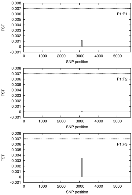
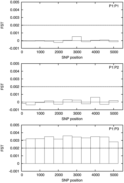
 is essentially zero everywhere except for a
small region approximately halfway along the chromosome. The horizontal
dotted line is the value of
is essentially zero everywhere except for a
small region approximately halfway along the chromosome. The horizontal
dotted line is the value of  .
.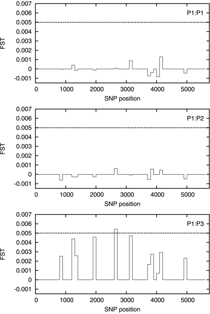
 . Note that
although
. Note that
although  is always
non-negative, the estimator may become negative for small values of
is always
non-negative, the estimator may become negative for small values of
 .
.
 .
.
 confidence
intervals.
confidence
intervals.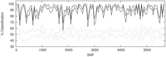
 confidence
intervals.
confidence
intervals.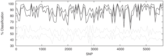
 confidence
intervals.
confidence
intervals.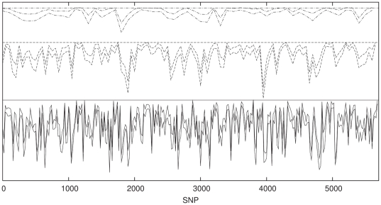
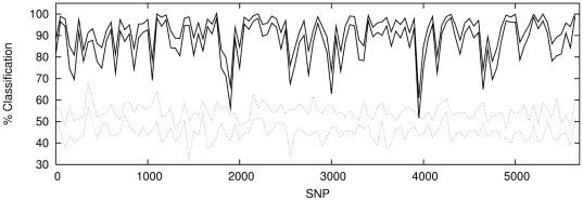
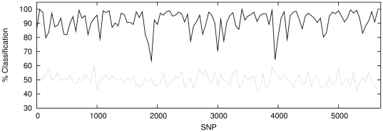
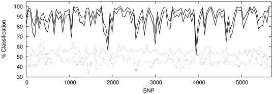
 classification in each case.
References
-
- Lao O, Lu T, NothNagel M, Junge O, Freitag-Wolf S, et al. Correlation Between Genetic and Geographic Structure in Europe. Curr Biol . 2008;18:1241–1248. - PubMed
-
- International Schizophrenia Consortium website. Available: http://pngu.mgh.harvard.edu/isc. Accessed 2011.
Publication types
MeSH terms
Grants and funding
LinkOut - more resources
Full Text Sources
