Dynamic linear model analysis of optical imaging data acquired from the human neocortex

Abstract

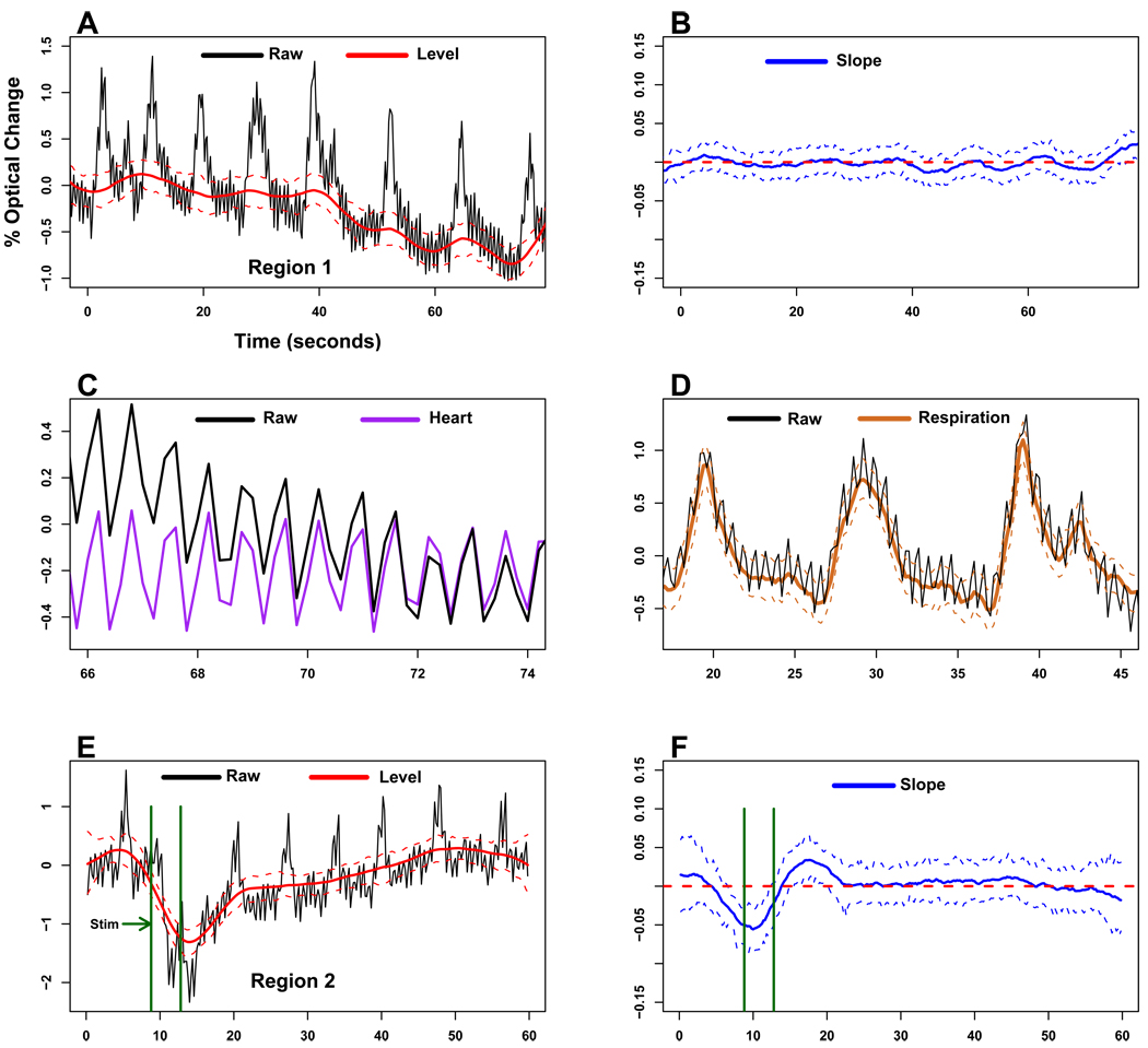
The amount of light absorbed and scattered by neocortical tissue is altered by neuronal activity. Imaging of intrinsic optical signals (ImIOS), a technique for mapping these activity-evoked optical changes with an imaging detector, has the potential to be useful for both clinical and experimental investigations of the human neocortex. However, its usefulness for human studies is currently limited because intraoperatively acquired ImIOS data is noisy. To improve the reliability and usefulness of ImIOS for human studies, it is desirable to find appropriate methods for the removal of noise artifacts and its statistical analysis. Here we develop a Bayesian, dynamic linear modeling approach that appears to address these problems. A dynamic linear model (DLM) was constructed that included cyclic components to model the heartbeat and respiration artifacts, and a local linear component to model the activity-evoked response. The robustness of the model was tested on a set of ImIOS data acquired from the exposed cortices of six human subjects illuminated with either 535nm or 660nm light. The DLM adequately reduced noise artifacts in these data while reliably preserving their activity-evoked optical responses. To demonstrate how these methods might be used for intraoperative neurosurgical mapping, optical data acquired from a single human subject during direct electrical stimulation of the cortex were quantitatively analyzed. This example showed that the DLM can be used to provide quantitative information about human ImIOS data that is not available through qualitative analysis alone.

Figure 1. Characteristics of Optical Imaging Data at 535 nm and 660 nm

A pseudo-colored map of the electrical stimulation-evoked optical changes over the cortical surface at 535 nm (panel A) shows that the largest changes occur in the tissue surrounding the stimulating electrodes (“S”, panel B). Visual comparison of the optical changes in panel A to the positions of the larger vessels identifiable in panel B shows that the activity-evoked optical changes at 535 nm are absent from such vessels. The largest optical changes at this wavelength are negative-going, showing a decrease in light absorption when compared to pre-stimulus conditions. In contrast to the changes at 535 nm, the largest optical changes at 660 nm (panel C) are restricted to one or more of the larger veins and are positive-going. Optical imaging data is analyzed by selecting at least nine regions of interest, each one consisting of approximately 5000 pixels, covering an area of 20 mm². Regions are selected over tissue areas from which larger vessels were absent (blue circles, panel B), or from segments overlying larger veins in which activity-evoked signals are observed to occur at 660 nm (red overlays, panel B). Time series of these optical data (blue and red plots, panels D and E) are generated by calculating the percent change (relative to a control image) of the average of the pixel values within each region for every image in an experimental trial. ECoG recordings (green traces, panels D and E) from surface electrodes (marked “R” in panel B) were simultaneously acquired with the optical data so that the timing of the electrical stimulus relative to the changes in the optical signal could be accurately determined from the stimulus-artifact, and to monitor for the presence of afterdischarges and spontaneous activity. Time series for regions from which the largest activity-evoked optical changes were elicited at 535 nm (Region 1; blue traces) and at 660 nm (Region 9; red traces) are shown in panels D and E. These plots show patterns of noise occurring at both wavelengths that include larger spikes with a period of approximately 5s due to respiration, along with smaller spikes with a period of 0.8 s due to heartbeat. The inset in the bottom left of panel D shows a smaller section of the 535 nm optical signal plotted at a slower time course and larger scale. Note that the amplitude and duration of each respiration and heartbeat artifact can vary between cycles. The optical response of Region 9 overlying the vein at 660 nm shown in panel E (red trace) is more complicated than the 535 responses of the tissue shown in panel D, with the shape of the initial response and the magnitude of the later fluctuations about the baseline difficult to accurately discern in the presence of the respiration and heartbeat artifacts.

Figure 2. Results of Model 1

The accuracy of the first DLM, Model 1, is assessed here by examining how well its estimated level, heartbeat, and respiration components match those of the real optical data. For this purpose, two time series of 530 nm optical data were chosen for analysis: Region 1 (panel A, black trace), from a control-experiment in which no electrical stimulus was given, and Region 2 (panel E, black trace), in which a small optical response (< 2%) appeared to be elicited by the stimulation that was applied from t = 8.8s to t = 12.8s (green vertical bars, panels E and F). Since no stimulus was applied to Region 1, the estimated level (linear trend) would be expected to be relatively flat, with perhaps some drift around the baseline value. However, the estimated level component for Region 1 (panel A, solid red line with 90% CIs shown as dotted red lines) appears to closely follow the respiration cycles. The estimated slope (i.e. rate of change, or derivative) of the level component for Region 1 (panel B, solid blue trace with 90% CIs plotted as dotted lines; dashed red line indicates where the slope is unchanging) confirms that significant changes are occurring with the estimated level component that coincide with the rising and falling of each respiration cycle. To study the accuracy of Model 1’s estimation of the heartbeat, the estimated heartbeat component and the raw data are plotted together at a slower time course and magnified scale (panel C; purple trace is the estimated heartbeat, black trace is raw data; CIs not shown for clarity). A similar plot comparing the model-estimated respiration component to the raw data is shown in panel D (solid brown trace is estimated respiration with 90% CIs shown as dotted lines, black trace is raw data). The respiration artifacts in the estimated level component and slope for Region 2 (panels E, F) similarly suggest that Model 1 does not accurately estimate the respiration component. The changes in the optical response elicited by the stimulus are not obviously distinguishable from the respiration artifacts in the slope (panel F).

Figure 3. Results of Model 2

Model 2 was constructed by modifying Model 1 to included an additional harmonic for the respiration component, while keeping all other details of Model 1 unchanged. The same time series that were analyzed in Figure 2 with Model 1 are again analyzed here with Model 2 (raw data plotted in panels A and E as black traces). The estimated level curves (panels A and E, solid red traces; 90% CIs indicated by dotted lines) have greatly reduced heartbeat and respiration artifacts. The estimated slope for Region 1 which was acquired during control conditions in which there was no electrical stimulation is relatively flat with small fluctuations around baseline (panel B; solid blue trace; 90% CIs indicated by dotted lines; red dashed line indicates where the slope is unchanging). Comparison of the estimated respiration component (panel D; brown trace) to the raw data (panel D; black trace) shows that Model 2 appears to accurately capture the complex shapes of the varying respiration cycles. The small optical response elicited by electrical stimulation in Region 2 is now evident (panel E, red traces), and its corresponding slope (panel F, blue traces; dashed red line indicates where the slope is unchanging) now shows a clear deviation from the baseline during the onset and recovery of the optical response to the stimulus.

Figure 4. Fourier Analysis of the Linear Trends Estimated by Models 1 and 2

To further understand the differences in the results given by the two DLMs, periodograms of their estimated level plots and of the raw data were compared. Panel A shows superimposed plots of the raw data (black trace) and level components given by Model 1 (red trace) and Model 2 (blue trace) for Region 2 (see Figures 2 and 3, panel E). The level estimated by Model 1 appears to be an accurate representation of the raw data, but with a complete filtering of the heartbeat cycles, leaving the respiration cycles unaltered to visual inspection. The level estimated by Model 2 appears to be a complete filtering of both the heartbeat and respiration cycles, while maintaining the stimulation-evoked optical response. The periodograms for each of the traces in panel A are shown below in panel B using the same colors for the corresponding traces. The periodogram for the raw data shows a large peak at the heartbeat frequency, marked by an asterisk in the black trace, that is absent in the level curve estimated by Model 1.

Figure 5. Analysis of Residuals from Model 2

The residuals given by the estimate of Model 2 for Region 2 are analyzed here. The raw residuals are shown in panel A with vertical dashed lines showing the interval over which the cortex was stimulated. The standardized residuals shown in panel B provides evidence that their distribution is Normal since approximately 95% lie between +/− 2. The Normal Q-Q plot in panel C provides further evidence that the residuals are normally distributed. The autocorrelation plot of the residuals shown in panel D (horizontal dashed lines show 95% confidence intervals) shows little significant autocorrelation. Normal Q-Q plots (not shown) for the residuals given by Model 2 were generated for 18 other regions selected from the 6 subjects studied here, all showing reasonable agreement with Normality.

Figure 6. Primate and Human Signals for Testing Accuracy of Model 2

Primate optical data showing a response to an electrical stimulus was combined with human data containing respiration and heartbeat artifacts (and no activity-evoked response) to test the accuracy of Model 2. Heartbeat artifacts can be removed from primate data using a running-mean filter of window-length 7 (covering about 1s of the time series at the frequency in which these data were acquired), without significantly altering any changes occurring at a lesser frequency in the raw data. The trace showing the largest optical response in the top panel illustrates this processing. The raw data is plotted as a black trace in which the high-frequency heartbeat artifact can be seen. The mean-filtered time series derived from the raw data is plotted as an overlying red trace. Four other similarly smoothed time series acquired from the primate are shown, chosen from regions at various distances from the stimulating electrode so that a variety of responses with different magnitudes and durations could be tested. Each of these time series was acquired with the application of four seconds of electrical stimulation to the cortex beginning at t = 20s. The noisy human data to be combined with each of the traces in the top panel is shown in the bottom panel (black trace). The estimated level component of this noisy trace given by Model 2 is overlaid as a red trace (thick line) with its 90% CIs (thinner lines), showing that only small fluctuations around the baseline are present in its linear trend.

Figure 7. Accuracy of Model 2 in Recovering Activity-evoked Optical Responses

The noisy human data containing heartbeat and respiration artifacts were combined with each of the five primate noise-free time series from the previous figure. The estimated level components given by Model 2 for each of these combined time series were then plotted in panels 1–5. Each panel shows the estimated levels and their 90% CI (black traces), with the original ‘true data’ overlaid (red trace), for each of the combined series. The plots in each panel are drawn at different scales determined by the minimum and maximum values of the individual time series. The primate data for panel 5 contains a small ‘wiggle’ during its peak response that is lost in the estimated level component. To understand the reason for this loss of accuracy, the combined [human noisy + primate] time series (black trace) is compared to the true signal (red trace) and the estimated level component (blue trace) in panel 6. It is apparent that the wiggle in the true data coincidentally is of a similar shape as the respiration cycles.

Figure 8. DLM Analysis of Optical Responses From Six Subjects at 535nm and 660nm

To further examine the applicability of the DLM analysis, we examined the estimated level components of time series acquired from six different subjects, at both 535 and 660 nm light. The bottom trace in panel A shows the optical response acquired at 535nm (level component, purple trace; raw data, black trace), the middle trace shows the optical response at 660nm (level component, purple trace; raw data, black trace) and the top trace shows the ECoG activity (blue trace) recorded during the acquisition of the 535 nm data. Vertical dotted lines show the interval during which the stimulus was applied to the cortex. Panels B through F show two pairs of time series for the raw data (black traces) with the overlaid level components for 535 nm (purple traces) and 660 nm (red traces). In order from bottom to top, the traces in each panel are from: i) The region showing the largest optical response to a given stimulus at 535 nm, ii) the smallest responding region at 535 nm, iii) the largest responding region at 660 nm, and iv) the smallest responding region at 660 nm. The optical responses in panels A–D were each elicited by four seconds of electrical simulation applied to the cortex, and those in panels E and F are functionally-evoked responses from regions overlying tongue motor-sensory cortex elicited by sensory activation. The pair of vertical dotted lines in each panel indicate the time during which the cortex was activated either by electrical stimulation or a tongue motor-sensory task.

Figure 9. Inferential Analysis of Optical Responses during Awake and Anesthetized States

The optical responses shown here were acquired from the cortex of a single subject during four stimulation-trials at each current of 4mA, 8mA, and 14 mA (for a total of twelve stimulation-trials). Two stimulations at each current were administered while the patient was awake, and two at each current while the patient was anesthetized. Top Left Panel: Optical imaging data has typically been represented qualitatively as pseudo-colored images, in which colors are assigned to pixels in some way so that different magnitudes of response can be visually distinguished. Shown in the upper left panel is a gray-scale image (left) and its pseudo-colored image (right) representing the largest optical response that was elicited by four seconds of 8 mA stimulation. The colors were assigned according to a ‘spectrum’ coloring scheme in which red is assigned to those pixels showing the largest magnitude changes (^~−12% in this image) and dark blue to those pixels undergoing small changes close to 0%. Two regions were selected for further analysis; Region-1 near the stimulating electrode (labeled “Stim”) around which the largest optical response was elicited, and Region 2 at a position 2 cm away from the stimulating electrode and on a different gyrus than Region 1. Right panels: The optical responses of the two regions to four seconds of stimulation current (blue traces) and during a control period when no stimulus was applied (black trace at the top near 0% in each plot) are plotted with their 90% CIs (red traces). Only one of the four level curves (estimated by Model 2) obtained at each of the stimulating currents is plotted for Region-1 (top) and Region-2 (bottom). Bottom left panel: The peak optical responses were estimated by using Model 2 to generate the posterior distributions for the peak response in the level component, and at each region (Region 1, red; Region 2, blue), for each of the twenty-four stimulation time series. That is, twelve stimulation trials were carried out for each region, with two stimulations at each of the three currents for both awake and anesthetized conditions.

References

1. Aguilar O, Huerta G, Prado R, West M. Bayesian inference on latent structure in time series. In: Bernardo JM, Berger JO, Dawid AP, Smith AFM, editors. Bayesian Statistics 6: Proceedings of the Sixth Valencia International Meeting; Oxford: Clarendon Press; 1999. pp. 3–26.
1. Bathellier B, Van De Ville D, Blu T, Unser M, Carleton A. Wavelet-based multi-resolution statistics for optical imaging signals: application to automated detection of odour activated glomeruli in the mouse olfactory bulb. NeuroImage. 2007;34:1020–1035. - PubMed
1. Besag J, Green P, Higdon D, Mengersen K. Bayesian computation and stochastic systems. Statist Sci. 1995;10:3–36.
1. Birn RM, Diamond JB, Smith MA, Bandettini PA. Separating respiratory-variation-related fluctuations from neuronal-activity-related fluctuations in fmri. Neuroimage. 2006;31:1536–1548. - PubMed
1. Cannestra AF, Pouratian N, Bookheimer SY, Martin NA, Beckerand DP, Toga AW. Temporal spatial differences observed by functional mri and human intraoperative optical imaging. Cereb Cortex. 2001;11:773–782. - PubMed
Publication types
LinkOut - more resources