MR perfusion imaging in acute ischemic stroke

Abstract

Magnetic resonance (MR) perfusion imaging offers the potential for measuring brain perfusion in acute stroke patients, at a time when treatment decisions based on these measurements may affect outcomes dramatically. Rapid advancements in both acute stroke therapy and perfusion imaging techniques have resulted in continuing redefinition of the role that perfusion imaging should play in patient management. This review discusses the basic pathophysiology of acute stroke, the utility of different kinds of perfusion images, and research on the continually evolving role of MR perfusion imaging in acute stroke care.

Figure 1. Dynamic susceptibility contrast (DSC) perfusion imaging

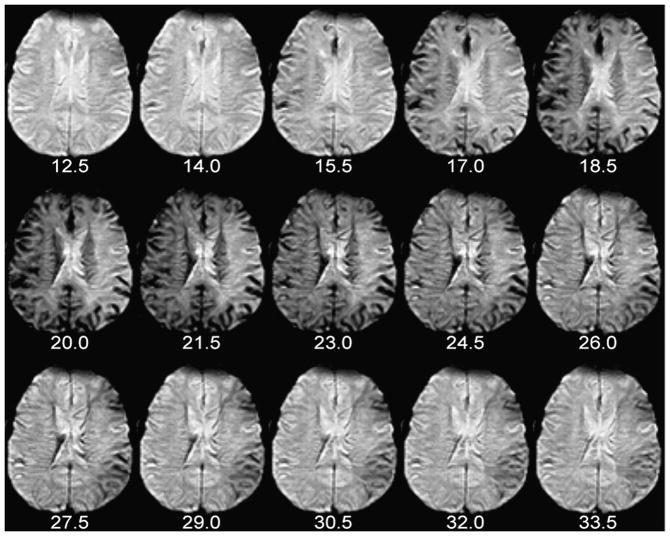
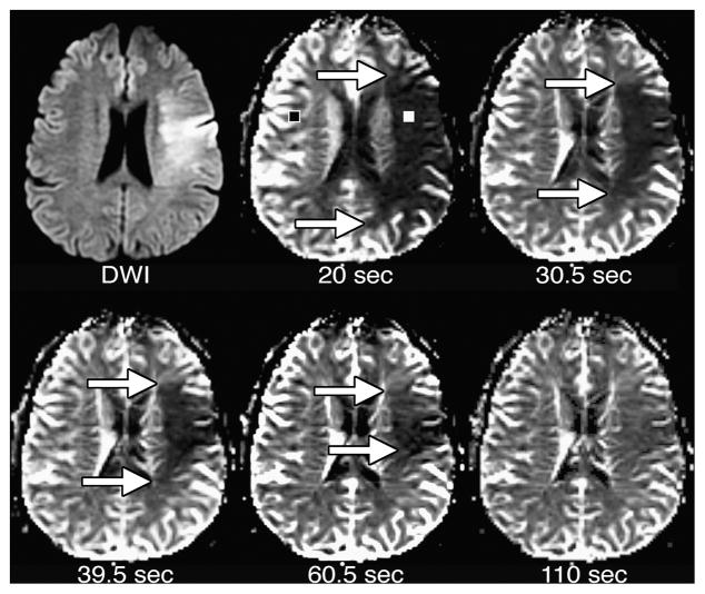
The number of seconds elapsed since the beginning of contrast injection appears beneath each image. Note the appearance of contrast in some large arteries, which become hypointense and “bloom” slightly, at 14.0 and 15.5 seconds post-injection (i.e. 24.0 and 25.5 seconds after the beginning of the scan). By 20.0 seconds post-injection, the presence of gadolinium in small vessels causes loss of parenchymal signal intensity in the normally perfused right hemisphere. Arrival of contrast is delayed and prolonged in the left hemisphere. These perfusion source images were used to create the graph and CBV maps in Figures 8 and 9, respectively.

Figure 2. Comparison of MR and CT perfusion imaging

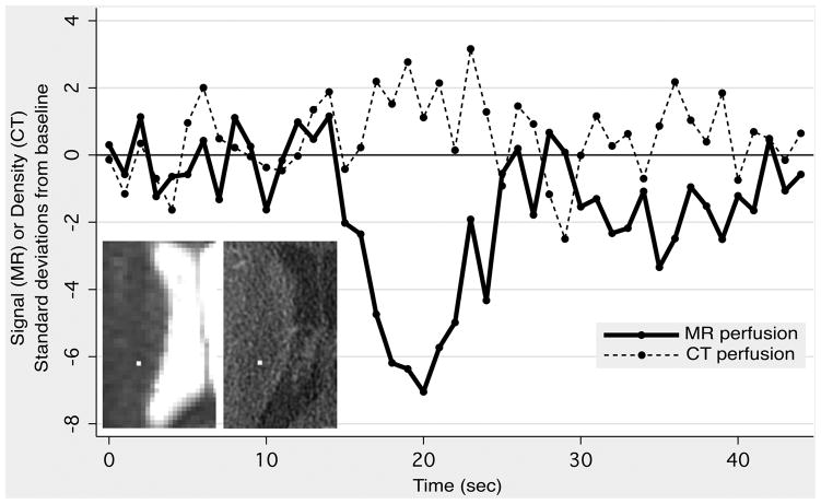
A 59-year-old male presented with slurred speech. DWI and CT angiography were normal, and the patient was subsequently diagnosed with ethanol intoxication. MR perfusion imaging (MRP) was performed 17 minutes after CT perfusion imaging (CTP). Identically sized regions of interest were placed on MRP (left inset, 1×1 pixel) and CTP (right inset, 4×4 pixels) source images in a randomly-selected location in the right corona radiata. The graph shows MR signal intensity and CT density as a function of time, with both expressed in terms of standard deviations above or below the mean value obtained from baseline images acquired before the arrival of the contrast bolus. Note the much larger signal change observed with MRP, compared to the changes observed with CTP, which are barely discernable from random noise fluctuations.

Figure 3. Delayed bolus arrival with preserved CPP

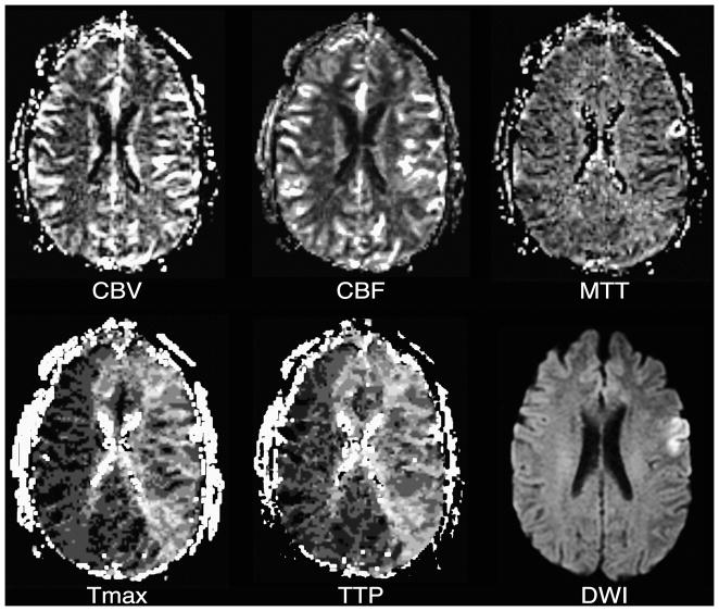
Tmax and TTP maps reflect delayed bolus arrival in most of the left cerebral hemisphere. Although there is the suggestion of slightly elevated CBF in some of the involved tissue, which could represent post-ischemic hyperperfusion, CBV, CBF, and MTT otherwise appear normal. A corresponding DWI image is presented for reference.

Figure 4. Compensated low CPP

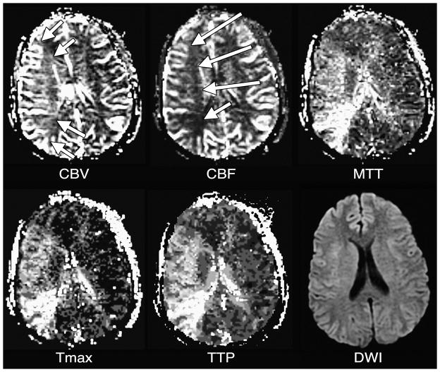
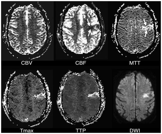
Elevated CBV (arrows) in the right middle cerebral artery territory reflects vasodilation in response to decreased CPP. The CBF map shows that this response has been successfully in maintaining apparently normal CBF (arrows). MTT is elevated in the affected tissue. The Tmax map shows delayed bolus arrival. TTP is prolonged, probably as a result of both delayed bolus arrival and increased MTT. A corresponding DWI image is presented for reference.

Figure 5. Hypoperfusion

CBF is decreased within a small wedge-shaped region in the left middle cerebral artery territory (arrows). There is a corresponding region of MTT prolongation (arrows). Tmax and TTP maps, as well as a DWI image, also show corresponding abnormalities.

Figure 6. Post-ischemic hyperperfusion

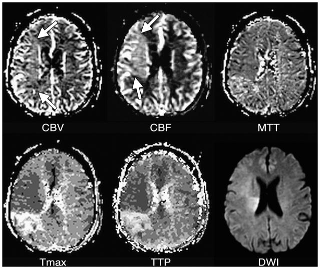
CBV is slightly elevated (arrows) in most of the right middle cerebral artery territory, reflecting vasodilation. In most of this tissue, CBF is higher than normal (arrows), demonstrating the vasodilation has persisted following an ischemic insult. MTT in this tissue may be minimally decreased in the hyperperfused tissue, although normal or elevated MTT are sometimes seen in such conditions. The Tmax map shows that bolus arrival is early in the hyperperfused tissue, although normal or (rarely) delayed arrival also can be seen in post-ischemic hyperperfusion. Post-ischemic hyperperfusion can occur in tissue that did or did not experience irreversible injury, as shown by the DWI image, in which some but not all of the hyperperfused tissue appears abnormal. Note that there is a persistently underperfused region posterior to the hyperperfused area.

Figure 7. TTP delay in varying hemodynamic conditions

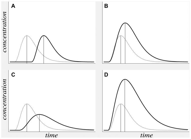
Theoretical concentration-versus-time curves (solid lines) reflect the four different abnormal hemodynamic conditions listed in Table 1: (A) delayed bolus arrival with preserved CPP, (B) compensated low CPP, (C) hypoperfusion, and (D) post-ischemic hyperperfusion. In each case, a concentration-versus-time curve for normal tissue is presented for comparison (dotted lines). TTP (vertical lines) can be delayed (i.e farther to the right) in all four conditions.

Figure 8. Effect of perfusion scan duration on calculated CBV

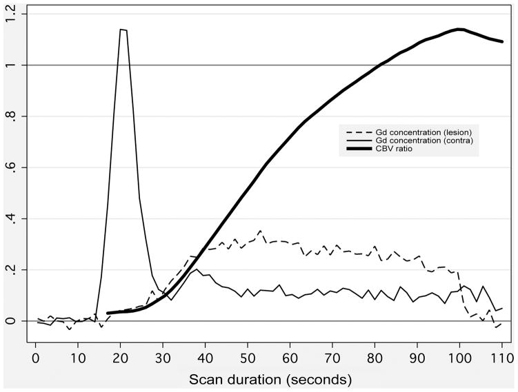
Thin lines depict gadolinium concentration (in arbitrary units) versus time following contrast injection, within small regions of interest (ROIs) placed in an acute stroke patient’s low-CBF lesion (thin dashed line), and in the corresponding location in the unaffected contralateral hemisphere (thin solid line). ROI locations are show in Figure 9. Because of low blood flow, the curve rises much more slowly in the low-CBF lesion. CBV in each ROI (not shown) is calculated as the area under the concentration-versus-time curve. Therefore, for simulated short scan durations, the ratio of CBV in the lesion to normal CBV (thick solid line) is far below unity. However, when longer, more accurate scan durations are used, the ratio rises above unity, showing that CBV is actually elevated in the low-CBF ROI.

Figure 9. Effect of perfusion scan duration on CBV maps

CBV maps were made from the perfusion data shown in Figures 1 and 8. Maps were made using the entire scan, which lasted 110 seconds after contrast injection, as well as truncated data sets simulating the effects of shorter scan durations lasting 20, 30.5, 39.5, and 60.5 seconds after contrast injection. With the shortest scan duration of 20 seconds, there is a region of very low apparent CBV, which is much larger than the DWI lesion. With progressively longer scan durations, the size of the apparent CBV lesion shrinks. With the full 110-second scan duration, there is only a poorly delineated region of slightly reduced CBV that is considerably smaller than the DWI lesion.

Figure 10. Effects of scan duration on various perfusion maps

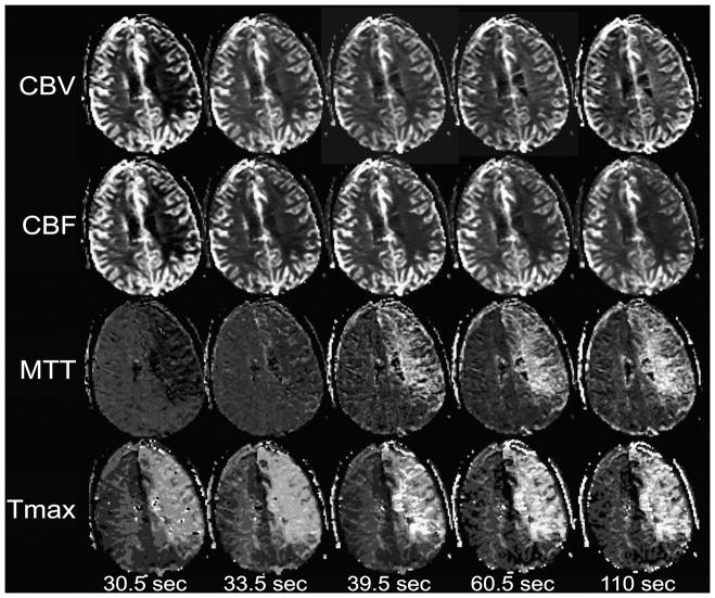
Perfusion maps were made from a patient other than those depicted in previous figures, using data from the entire scan lasting 110 seconds after contrast injection, as well as temporally truncated subsets of the data simulating shorter scan durations. With the shortest scan duration of 30.5 seconds, there is a large low-CBV lesion occupying most of the left cerebral hemisphere. The apparent severity of CBV reduction is decreased with the 33.5-second scan, and no CBV lesion is apparent with the 39.5-second scan. With the 60.5- and 110-second scans, it is apparent that CBV is mildly elevated in the left hemisphere. CBF is artifactually reduced with the 30.5-second scan, but does not change significantly in the longer scans. Because MTT is calculated as the quotient of CBV divided by CBF, the effect of scan duration on CBV results in apparently reduced MTT with the shortest scan duration, and no obvious MTT lesion at 33.5 seconds, although a large region of prolonged MTT is clearly evident with longer scan durations. Tmax is not significantly changed by scan duration. DWI (not shown) was normal in this part of the brain.

Figure 11. CBF, Tmax and convolution

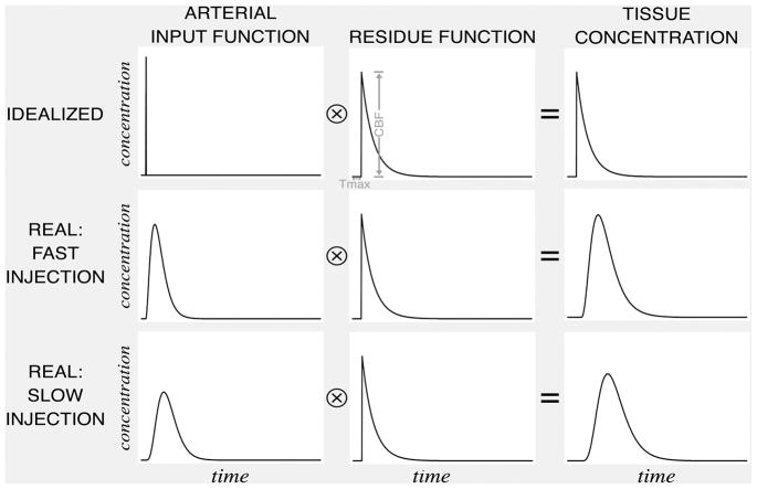
Each voxel has a “residue function” reflecting the proportion of an idealized, instantaneously injected unit-sized contrast bolus that remains in the voxel following its arrival. The tissue concentration function is the convolution of the arterial input function (which varies depending on complex variables such as contrast bolus injection rate, cardiac output, and patient anatomy), and a multiple of the residue function that has been scaled by the value of CBF. The amplitude of this scaled residue function is CBF, and the time at which it reaches its maximum is Tmax. The scaled residue function cannot be observed directly. If both the concentration function and an arterial input function are known, the scaled residue function can be calculated by deconvolution.

References

-
- Rosen BR, Belliveau JW, Chien D. Perfusion imaging by nuclear magnetic resonance. Magn Reson Q. 1989;5:263–281. - PubMed
- Powers WJ. Cerebral hemodynamics in ischemic cerebrovascular disease. Ann Neurol. 1991;29:231–240. - PubMed
- Grubb RL, Jr, Phelps ME, Ter-Pogossian MM. Regional cerebral blood volume in humans. X-ray fluorescence studies. Arch Neurol. 1973;28:38–44. - PubMed
- Grubb RL, Jr, Phelps ME, Raichle ME, Ter-Pogossian MM. The effects of arterial blood pressure on the regional cerebral blood volume by x-ray fluorescence. Stroke. 1973;4:390–399. - PubMed
Publication types
MeSH terms
Grants and funding
LinkOut - more resources
Full Text Sources
Other Literature Sources