Visualizing fitness landscapes

Abstract

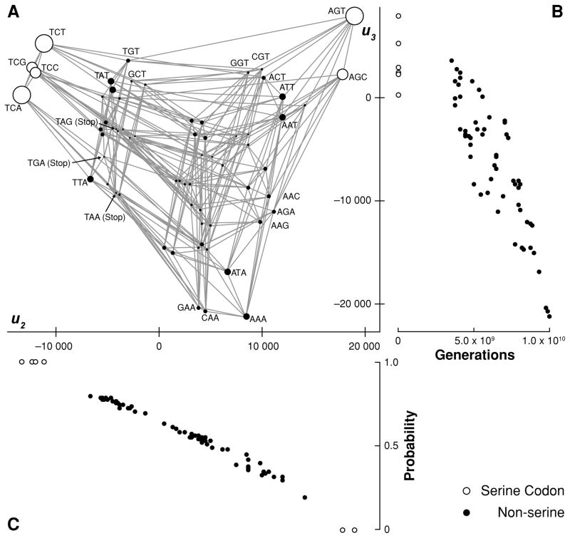
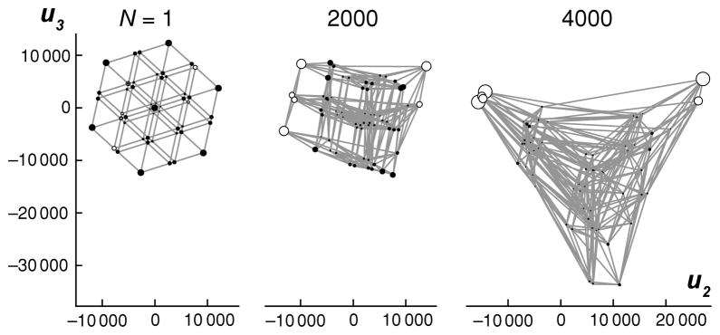
Fitness landscapes are a classical concept for thinking about the relationship between genotype and fitness. However, because the space of genotypes is typically high-dimensional, the structure of fitness landscapes can be difficult to understand and the heuristic approach of thinking about fitness landscapes as low-dimensional, continuous surfaces may be misleading. Here, I present a rigorous method for creating low-dimensional representations of fitness landscapes. The basic idea is to plot the genotypes in a manner that reflects the ease or difficulty of evolving from one genotype to another. Such a layout can be constructed using the eigenvectors of the transition matrix describing the evolution of a population on the fitness landscape when mutation is weak. In addition, the eigendecomposition of this transition matrix provides a new, high-level view of evolution on a fitness landscape. I demonstrate these techniques by visualizing the fitness landscape for selection for the amino acid serine and by visualizing a neutral network derived from the RNA secondary structure genotype-phenotype map.

Figure 1

A one codon fitness landscape with selection for serine and against stop codons. The six serine codons have fitness 1.001, the three stop codons have fitness .999, all other codons have fitness 1.000, N = 3000, natural selection is modeled as a Moran process, and mutation is based on empirically observed rates for yeast (Lynch et al., 2008). (A) Genotypes coding for serine are shown as unfilled circles, all other genotypes are shown as filed circles, and the area of each circle is proportional to its frequency at equilibrium. Edges connect genotypes that differ by a single point mutation. (B) The u₃ coordinate of each genotype is plotted against the expected number of generations before a population starting at that genotype would evolve a serine. (C) The probability that a population starting at a given genotype evolves a serine coded for by TCA, TCG, TCC, or TCT before evolving a serine coded for by AGT or AGC is plotted against the u₂ coordinate of that genotype.

Figure 2

The fitness landscape from Fig. 1A is shown for three different population sizes, N. For N = 1, the representation is highly symmetric, reflecting the neutral population dynamics. As N increases, the representation becomes increasingly deformed, reflecting the increasing power of natural selection. Notice that for increasing N, the equilibrium frequency of codons coding for serine increases (unfilled circles), and the distance between the two fitness peaks also increases, reflecting the longer waiting time for deleterious fixations.

Figure 3

A neutral network from the RNA sequence to RNA secondary structure genotype-phenotype map previously studied by van Nimwegen et al. (1999). 51 028 single stranded RNA sequences of length 18 are shown, each of which folds into the same secondary structure. The visualization was produced by assuming that each possible point mutation occurs with probability 1/1000 per generation, that all sequences with the target secondary structure are of equal fitness, and that only such sequences are viable. The sequences fall into 3 clusters (shown by the range bars at the top of the figure), which correspond to the possible base identities for the basepair formed between the 2nd and 17th bases. In the inset, genotypes are colored according to their equilibrium frequency in the strong mutation regime. Genotypes whose occupation is greater than 2.0 × 10⁻⁵ = 1/51 028 are shown in black.

References

1. Ashlock D, Schonfeld J. Proceedings of the 2005 Congress on Evolutionary Computation. Vol. 3. Springer; 2005. Nonlinear projection for the display of high dimensional distance data; pp. 2776–2783.
1. Barton NH, Coe JB. On the application of statistical physics to evolutionary biology. J Theor Biol. 2009;259:317–324. - PubMed
1. Belkin M, Niyogi P. Laplacian eigenmaps for dimensionality reduction and data representation. Neural Comput. 2003;15:1373–1396.
1. Berger MF, Philippakis AA, Qureshi AM, He FS, Estep PW, III, Bulyk ML. Compact, universal DNA microarrays to comprehensively determine transcription-factor binding site specificities. Nat Biotechnol. 2006;24:1429–1435. - PMC - PubMed
1. Bornberg-Bauer E, Chan HS. Modeling evolutionary landscapes: mutational stability, topology, and superfunnels in sequence space. Proc Natl Acad Sci USA. 1999;96:10689. - PMC - PubMed
Publication types