Cactus: Algorithms for genome multiple sequence alignment

Abstract

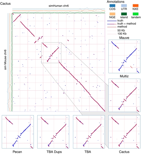
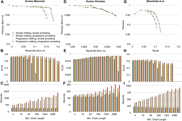
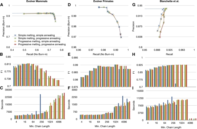
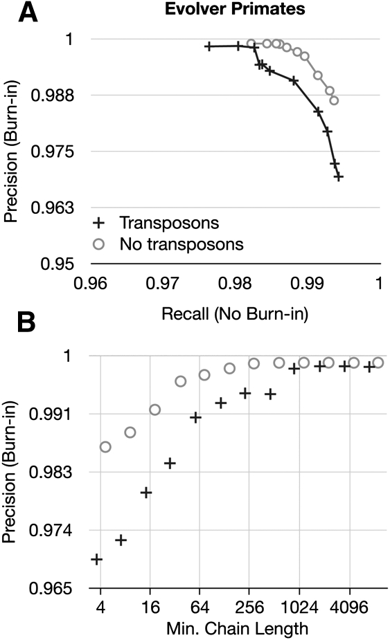
Much attention has been given to the problem of creating reliable multiple sequence alignments in a model incorporating substitutions, insertions, and deletions. Far less attention has been paid to the problem of optimizing alignments in the presence of more general rearrangement and copy number variation. Using Cactus graphs, recently introduced for representing sequence alignments, we describe two complementary algorithms for creating genomic alignments. We have implemented these algorithms in the new "Cactus" alignment program. We test Cactus using the Evolver genome evolution simulator, a comprehensive new tool for simulation, and show using these and existing simulations that Cactus significantly outperforms all of its peers. Finally, we make an empirical assessment of Cactus's ability to properly align genes and find interesting cases of intra-gene duplication within the primates.

Figure 1.

(A) A column containing four positions: X_i, −X_j, −Y_k, and Z_l. The overlaid trees show the position's phylogenetic relationships. (B) The mirror of the column in A. (C) A most parsimonious history for the base pairs in A. A substitution is inferred to have occurred along the lineage marked by a star, but the base pairs are all still considered homologous. (D) The mirror history of C.

Figure 2.

(A) An adjacency graph G₀ showing examples of threads. Blue and green lines depict two homologous threads traversing a series of residues in blocks and the joining adjacencies. The block edges are the aligned boxes containing letters. The stub edges are the aligned boxes not containing letters. The ends of the blocks/stubs are mapped as filled black rectangles on the edges of the aligned boxes. The adjacency edges are sets of lines connecting nodes. To distinguish the backdoor adjacencies, they are dotted. DNA bases within the adjacencies are written along the lines representing adjacency edges. Starting at a₁, the blue thread gives the sequence ACTTAGAATTCATTTTGCCTGGAGGCTCTGTGGATGAC. Similarly, the green thread gives the sequence AGCCTGCATAGAAGTCATggCATTTGTGAAggCTGATTCccctaAG. The lowercase letters represent the reverse complement of the block residues and adjacency sequences as they are written, and result from the traversal of the adjacency/block in the reverse orientation from right to left. (B) The Cactus graph G for G₀. The blue and green lines again depict the two threads. Each node is shown as a circle; the origin node is colored gray. The block/stub edges are depicted with multiple arrows, representing the different threads traversing them. Stub edges are dotted. The red numbers indicate the length of the chains. (C) The Cactus graph with embedded net substructure (G₀, G). Each node in (G₀, G) has added adjacency edges drawn, which connect the block end nodes represented by the ends of the block edges incident with each node. The origin node in (G₀, G) is drawn containing the origin node from G₀ to connect the prefix and suffix adjacency substructure.

Figure 3.

Melting and annealing examples. (A) An example showing the results of melt((G₀, G), X), where (G₀, G) is the Cactus graph in Figure 2C and X = {c}. (B) Like A, but with chain g also removed. (C,D) Examples of the effect of anneal((G₀, G), ∼∼), where (G₀, G) are the Cactus graphs in B and ∼∼ contains the alignments in chain c of the Cactus graph in Figure 2B added. (E) The MSLC solution for the Cactus graph in Figure 2C with large chain threshold α = 8. This is the result of the annealing function illustrated by C and D. The length of the longest chain in B increases by 2.

Figure 4.

An illustration of the BAR algorithm. (A) A subgraph of an adjacency subgraph. The magenta and orange coloring of the blocks highlights the two chains; the outer A chain contains the inner B chain, which has been inverted in the red thread. (B) An example of the BAR algorithm. Box (1), four end alignments are constructed, one for each end in the net that contains ends of A and B. The alignments are oriented from their respective ends. These four alignments are inconsistent; if they were accepted as they are, they would together create many likely spurious alignments. Box (i), the blue adjacency sequence ACAT between a₁ and b₁, is chosen at random. A cut point is chosen (drawn as a red line) on an induced alignment, one containing only the columns with residues in the chosen adjacency sequence. The cut point must lie before the first, after the last, or between two residues in the adjacency sequence. The cumulative alignment score of aligned pairs to the adjacency sequence is shown below the two induced alignments, in both cases cumulated away from the respective block end. The cut point is chosen so that the cumulated score before the cut point in the induced alignment of a₁ plus the cumulated score after the cut point in the induced alignment of b₁ is maximal. Alignments to the adjacency sequence in the a₁ end alignment after the cut points are removed, and alignments to the adjacency sequence in the b₁ alignment before the cut points are removed. In this case, the cut point is after position 4, so all of the a₁ alignments are kept and all of the alignments to the adjacency sequence in the b₁ alignment are removed. Box (2), the result of removing the alignments discarded in (i). Boxes (ii–vi) and (3–7) show this process repeated for each of the remaining adjacency sequences in turn. The ordering of adjacency sequences in this process is random. (C) The resulting adjacency subgraph after the alignments in Box (7) of B are included. The adjacency sequences are now all empty, and there are three chains, the orange and magenta chains, which have been lengthened, and a single block cyan chain corresponding to an indel.

Figure 5.

A dot plot showing the Evolver mammals alignment of simMouse and simHuman. The true alignment is shown in blue, and overlaid in red is the predicted Cactus alignment. The density of different sequence annotations, as maintained by the Evolver model, are plotted on rows along the axes. (CDS) Coding sequence; (UTR) untranslated region; (NXE) non-exonic conserved regions; (NGE) non-genic conserved regions; (island) CpG islands; (tandem) repetitive elements. The gray box is expanded at the bottom of the figure for five different predicted alignments. Only the Cactus alignment correctly identifies the tandem duplication at the bottom left of the expanded region.

Figure 6.

The effects of altering the minimum chain length α on the alignment predicted by the CAF algorithm. (A–C) Using the Evolver mammals data set. (D–F) Using the Evolver primates data set. (G–I) Using the Blanchette data set. (A,D,G) Precision-recall plots. The variable α is altered in powers of 2 from 4 to 8192. In general, increasing α increases precision and decreases recall. Four strategies are shown, for the four combinations involving simple melting/progressive melting and simple annealing/progressive annealing. (B,E,H) The F_0.25 score (weighting precision fourfold over recall) as a function of α, for the four CAF strategies (colors consistent with [A,D,G]). (C,F,I) The computation time (using a single contemporary 0 × 86 processor) as a function of α.

Figure 7.

The effects of altering the minimum chain length α on the combined results of the CAF and BAR algorithms (the implementation is collectively called Cactus). The format of the figure is the same as in Figure 6, except F₁ scores are shown in plots B, E, and H.

Figure 8.

Comparing the effect of removing the repetitive transposition operation on two independent runs of the Evolver primates simulation, one including and one without the operation. (A) A precision-recall plot of the predicted Cactus alignments showing the effect of altering α in powers of 2 from 4 to 8192. (B) The precision as a function of α. Note particularly the step-up in precision between α = 512 and α = 1024 for the simulation including repetitive transposition, whose alignment is not considered homologous by Evolver.

Figure 9.

The effects of adjusting tree coverage. (A) A precision-recall plot of the predicted Cactus alignments showing the effect of altering α in powers of 2 from 4 to 8192. Four curves are plotted, showing changes in minimum tree coverage from 0 to 1.0 (see key in A). (B) The F₁ score as a function of α for the four different minimum tree coverages (colors consistent with A). (C) As in B, but showing time.

Figure 10.

The effect of adjusting γ. (A) A precision-recall plot of the predicted Cactus alignments showing the effect of altering γ, for the three different alignment simulations. (B) The F₁ score as a function of γ for the three different simulations; shapes consistent with A.

References

1. Blanchette M, Green ED, Miller W, Haussler D 2004a. Reconstructing large regions of an ancestral mammalian genome in silico. Genome Res 14: 2412–2423 - PMC - PubMed
1. Blanchette M, Kent WJ, Riemer C, Elnitski L, Smit AFA, Roskin KM, Baertsch R, Rosenbloom K, Clawson H, Green ED, et al. 2004b. Aligning multiple genomic sequences with the threaded blockset aligner. Genome Res 14: 708–715 - PMC - PubMed
1. Bradley RK, Roberts A, Smoot M, Juvekar S, Do J, Dewey C, Holmes I, Pachter L 2009. Fast statistical alignment. PLoS Comput Biol 5: e1000392 doi: 10.1371/journal.pcbi.1000392 - PMC - PubMed
1. Bray N, Pachter L 2004. Mavid: Constrained ancestral alignment of multiple sequences. Genome Res 14: 693–699 - PMC - PubMed
1. Brudno M, Do CB, Cooper GM, Kim MF, Davydov E, Program NCS, Green ED, Sidow A, Batzoglou S 2003a. Lagan and multi-lagan: Efficient tools for large-scale multiple alignment of genomic DNA. Genome Res 13: 721–731 - PMC - PubMed
Publication types
LinkOut - more resources